Microsoft Office Excel 2010 For Dummies

Greg Harvey, PhD
Bestselling author of Excel
All-in-One For Dummies
Learn to:
• Create and edit worksheets, format cells,
and enter formulas
• Add data tables and sort and filter records
• Create powerful charts with graphics
• Share worksheets via e-mail
and SharePoint
®
Excel
®
2010
Microsoft
®
Making Everything Easier!
™

Start with FREE Cheat Sheets
Cheat Sheets include
• Checklists
• Charts
• Common Instructions
• And Other Good Stuff!
Get Smart at Dummies.com
Dummies.com makes your life easier with 1,000s
of answers on everything from removing wallpaper
to using the latest version of Windows.
Check out our
• Videos
• Illustrated Articles
• Step-by-Step Instructions
Plus, each month you can win valuable prizes by entering
our Dummies.com sweepstakes. *
Want a weekly dose of Dummies? Sign up for Newsletters on
• Digital Photography
• Microsoft Windows & Office
• Personal Finance & Investing
• Health & Wellness
• Computing, iPods & Cell Phones
• eBay
• Internet
• Food, Home & Garden
Find out “HOW” at Dummies.com
*Sweepstakes not currently available in all countries; visit Dummies.com for official rules.
Get More and Do More at Dummies.com
®
To access the Cheat Sheet created specifically for this book, go to
www.dummies.com/cheatsheet/excel2010

Excel
®
2010
FOR
DUMmIES
‰


by Greg Harvey, PhD
Excel
®
2010
FOR
DUMmIES
‰

Excel
®
2010 For Dummies
®
Published by
Wiley Publishing, Inc.
111 River Street
Hoboken, NJ 07030-5774
www.wiley.com
Copyright © 2010 by Wiley Publishing, Inc., Indianapolis, Indiana
Published by Wiley Publishing, Inc., Indianapolis, Indiana
Published simultaneously in Canada
No part of this publication may be reproduced, stored in a retrieval system or transmitted in any form or
by any means, electronic, mechanical, photocopying, recording, scanning or otherwise, except as permit-
ted under Sections 107 or 108 of the 1976 United States Copyright Act, without either the prior written
permission of the Publisher, or authorization through payment of the appropriate per-copy fee to the
Copyright Clearance Center, 222 Rosewood Drive, Danvers, MA 01923, (978) 750-8400, fax (978) 646-8600.
Requests to the Publisher for permission should be addressed to the Permissions Department, John Wiley
& Sons, Inc., 111 River Street, Hoboken, NJ 07030, (201) 748-6011, fax (201) 748-6008, or online at http://
www.wiley.com/go/permissions.
Trademarks: Wiley, the Wiley Publishing logo, For Dummies, the Dummies Man logo, A Reference for the
Rest of Us!, The Dummies Way, Dummies Daily, The Fun and Easy Way, Dummies.com, Making Everything
Easier,
and related trade dress are trademarks or registered trademarks of John Wiley & Sons, Inc. and/
or its af liates in the United States and other countries, and may not be used without written permission.
Excel is a registered trademark of Microsoft Corporation in the United States and/or other countries. All
other trademarks are the property of their respective owners. Wiley Publishing, Inc., is not associated
with any product or vendor mentioned in this book.
LIMIT OF LIABILITY/DISCLAIMER OF WARRANTY: THE PUBLISHER AND THE AUTHOR MAKE NO
REPRESENTATIONS OR WARRANTIES WITH RESPECT TO THE ACCURACY OR COMPLETENESS OF
THE CONTENTS OF THIS WORK AND SPECIFICALLY DISCLAIM ALL WARRANTIES, INCLUDING WITH-
OUT LIMITATION WARRANTIES OF FITNESS FOR A PARTICULAR PURPOSE. NO WARRANTY MAY BE
CREATED OR EXTENDED BY SALES OR PROMOTIONAL MATERIALS. THE ADVICE AND STRATEGIES
CONTAINED HEREIN MAY NOT BE SUITABLE FOR EVERY SITUATION. THIS WORK IS SOLD WITH THE
UNDERSTANDING THAT THE PUBLISHER IS NOT ENGAGED IN RENDERING LEGAL, ACCOUNTING, OR
OTHER PROFESSIONAL SERVICES. IF PROFESSIONAL ASSISTANCE IS REQUIRED, THE SERVICES OF
A COMPETENT PROFESSIONAL PERSON SHOULD BE SOUGHT. NEITHER THE PUBLISHER NOR THE
AUTHOR SHALL BE LIABLE FOR DAMAGES ARISING HEREFROM. THE FACT THAT AN ORGANIZATION
OR WEBSITE IS REFERRED TO IN THIS WORK AS A CITATION AND/OR A POTENTIAL SOURCE OF FUR-
THER INFORMATION DOES NOT MEAN THAT THE AUTHOR OR THE PUBLISHER ENDORSES THE INFOR-
MATION THE ORGANIZATION OR WEBSITE MAY PROVIDE OR RECOMMENDATIONS IT MAY MAKE.
FURTHER, READERS SHOULD BE AWARE THAT INTERNET WEBSITES LISTED IN THIS WORK MAY HAVE
CHANGED OR DISAPPEARED BETWEEN WHEN THIS WORK WAS WRITTEN AND WHEN IT IS READ.
For general information on our other products and services, please contact our Customer Care
Department within the U.S. at 877-762-2974, outside the U.S. at 317-572-3993, or fax 317-572-4002.
For technical support, please visit www.wiley.com/techsupport.
Wiley also publishes its books in a variety of electronic formats. Some content that appears in print may
not be available in electronic books.
Library of Congress Control Number: 2010923559
ISBN: 978-0-470-48953-6
Manufactured in the United States of America
10 9 8 7 6 5 4 3 2 1
About the Author
Greg Harvey has authored tons of computer books, the most recent being
Excel Workbook For Dummies and Roxio Easy Media Creator 8 For Dummies,
and the most popular being Excel 2003 For Dummies and Excel 2003 All-in-One
Desk Reference For Dummies. He started out training business users on how
to use IBM personal computers and their attendant computer software in the
rough and tumble days of DOS, WordStar, and Lotus 1-2-3 in the mid-80s of
the last century. After working for a number of independent training rms,
Greg went on to teach semester-long courses in spreadsheet and database
management software at Golden Gate University in San Francisco.
His love of teaching has translated into an equal love of writing. For Dummies
books are, of course, his all-time favorites to write because they enable him
to write to his favorite audience: the beginner. They also enable him to use
humor (a key element to success in the training room) and, most delightful of
all, to express an opinion or two about the subject matter at hand.
Greg received his doctorate degree in Humanities in Philosophy and Religion
with a concentration in Asian Studies and Comparative Religion last May.
Everyone is glad that Greg was nally able to get out of school before he
retired.

Dedication
An Erucolindo melindonya

Author’s Acknowledgments
Let me take this opportunity to thank all the people, both at Wiley Publishing,
Inc., and at Mind over Media, Inc., whose dedication and talent combined to
get this book out and into your hands in such great shape.
At Wiley Publishing, Inc., I want to thank Andy Cummings and Katie Feltman
for their encouragement and help in getting this project underway and their
ongoing support every step of the way. These people made sure that the
project stayed on course and made it into production so that all the talented
folks on the production team could create this great nal product.
At Mind over Media, I want to thank Christopher Aiken for his review of the
updated manuscript and invaluable input and suggestions on how best to
restructure the book to accommodate all the new features and, most impor-
tantly, present the new user interface.

Publisher’s Acknowledgments
We’re proud of this book; please send us your comments at http://dummies.custhelp.com.
For other comments, please contact our Customer Care Department within the U.S. at 877-762-2974,
outside the U.S. at 317-572-3993, or fax 317-572-4002.
Some of the people who helped bring this book to market include the following:
Acquisitions and Editorial
Project Editor: Nicole Sholly
Senior Acquisitions Editor: Katie Feltman
Copy Editor: Brian Walls
Technical Editors: Mike Talley,
Joyce Nielsen
Editorial Manager: Kevin Kirschner
Editorial Assistant: Amanda Graham
Senior Editorial Assistant: Cherie Case
Cartoons: Rich Tennant
(www.the5thwave.com)
Composition Services
Project Coordinator: Patrick Redmond
Layout and Graphics: Ashley Chamberlain,
Joyce Haughey, Christine Williams
Proofreader: Linda Seifert
Indexer: Sharon Shock
Publishing and Editorial for Technology Dummies
Richard Swadley, Vice President and Executive Group Publisher
Andy Cummings, Vice President and Publisher
Mary Bednarek, Executive Acquisitions Director
Mary C. Corder, Editorial Director
Publishing for Consumer Dummies
Diane Graves Steele, Vice President and Publisher
Composition Services
Debbie Stailey, Director of Composition Services

Contents at a Glance
Introduction ................................................................ 1
Part I: Getting In on the Ground Floor ........................... 9
Chapter 1: The Excel 2010 User Experience .................................................................11
Chapter 2: Creating a Spreadsheet from Scratch ........................................................ 49
Part II: Editing without Tears ..................................... 95
Chapter 3: Making It All Look Pretty ............................................................................. 97
Chapter 4: Going Through Changes ............................................................................ 145
Chapter 5: Printing the Masterpiece ........................................................................... 175
Part III: Getting Organized and Staying That Way ..... 199
Chapter 6: Maintaining the Worksheet .......................................................................201
Chapter 7: Maintaining Multiple Worksheets .............................................................229
Part IV: Digging Data Analysis ................................. 253
Chapter 8: Doing What-If Analysis ............................................................................... 255
Chapter 9: Playing with Pivot Tables ..........................................................................267
Part V: Life beyond the Spreadsheet .......................... 283
Chapter 10: Charming Charts and Gorgeous Graphics ............................................. 285
Chapter 11: Getting on the Data List ........................................................................... 319
Chapter 12: Linking, Automating, and Sharing Spreadsheets .................................. 345
Part VI: The Part of Tens .......................................... 363
Chapter 13: Top Ten Features in Excel 2010 ..............................................................365
Chapter 14: Top Ten Beginner Basics ......................................................................... 369
Chapter 15: The Ten Commandments of Excel 2010 ................................................. 371
Index ...................................................................... 373


Table of Contents
Introduction ................................................................. 1
About This Book .............................................................................................. 1
How to Use This Book ..................................................................................... 2
What You Can Safely Ignore ........................................................................... 2
Foolish Assumptions ....................................................................................... 2
How This Book Is Organized .......................................................................... 3
Part I: Getting In on the Ground Floor ................................................. 3
Part II: Editing without Tears ...............................................................3
Part III: Getting Organized and Staying That Way .............................3
Part IV: Digging Data Analysis .............................................................. 4
Part V: Life beyond the Spreadsheet ................................................... 4
Part VI: The Part of Tens ....................................................................... 4
Conventions Used in This Book ..................................................................... 4
Icons Used in This Book ................................................................................6
Where to Go from Here ................................................................................... 6
Part I: Getting In on the Ground Floor ............................ 9
Chapter 1: The Excel 2010 User Experience . . . . . . . . . . . . . . . . . . . . . .11
Excel’s Ribbon User Interface ...................................................................... 12
Going Backstage via File......................................................................13
Bragging about the Ribbon ................................................................. 14
Customizing the Quick Access toolbar ............................................. 18
Having fun with the Formula bar .......................................................22
What to do in the Worksheet area ..................................................... 23
Showing off the Status bar .................................................................. 27
Launching and Quitting Excel ...................................................................... 28
Starting Excel from the Start menu....................................................28
Starting Excel from the Windows XP Start menu ............................. 29
Pinning a Microsoft Excel 2010 option
on your Windows Start menu ........................................................ 29
Adding a Microsoft Excel 2010 shortcut
to your Windows desktop ...............................................................30
Adding Excel to the Windows Quick Launch toolbar......................31

Excel 2010 For Dummies
xii
Pinning an Excel icon to the Windows 7 taskbar ............................. 31
Exiting Excel ......................................................................................... 32
Help Is on the Way ......................................................................................... 32
Migrating to Excel 2010 from Earlier Versions
Using Pull-down Menus ............................................................................. 33
Cutting the Ribbon down to size........................................................34
Finding the Standard toolbar buttons equivalents..........................39
Finding the Formatting toolbar buttons equivalents ......................42
Putting the Excel Quick Access toolbar
to good use during the transition .................................................. 43
Getting good to go with Excel 2010 ................................................... 47
Chapter 2: Creating a Spreadsheet from Scratch. . . . . . . . . . . . . . . . . .49
So What Ya Gonna Put in That New Workbook of Yours? ....................... 50
The ins and outs of data entry ...........................................................50
You must remember this . . . ..............................................................51
Doing the Data-Entry Thing .......................................................................... 51
It Takes All Types .......................................................................................... 53
The telltale signs of text ...................................................................... 54
How Excel evaluates its values .......................................................... 55
Fabricating those fabulous formulas! ................................................ 62
If you want it, just point it out ............................................................ 64
Altering the natural order of operations ..........................................65
Formula ub-ups .................................................................................. 66
Fixing Those Data Entry Flub-Ups ............................................................... 67
You really AutoCorrect that for me ................................................... 68
Cell editing etiquette ...........................................................................69
Taking the Drudgery out of Data Entry ....................................................... 71
I’m just not complete without you.....................................................71
Fill ’er up with AutoFill ........................................................................ 72
Inserting special symbols ...................................................................78
Entries all around the block ...............................................................79
Data entry express ............................................................................... 80
How to Make Your Formulas Function Even Better .................................. 80
Inserting a function into a formula with
the Insert Function button ..............................................................81
Editing a function with the Insert Function button .........................84
I’d be totally lost without AutoSum ................................................... 85
Making Sure That the Data Is Safe and Sound ...........................................87
The Save As dialog box in Windows 7 and Windows Vista ............88
The Save As dialog box in Windows XP ............................................ 89
Changing the default le location ...................................................... 90
The difference between the XLSX and XLS le format .................... 90
Saving the Workbook as a PDF File ............................................................. 91
Document Recovery to the Rescue ............................................................. 92

xiii
Table of Contents
Part II: Editing without Tears ...................................... 95
Chapter 3: Making It All Look Pretty. . . . . . . . . . . . . . . . . . . . . . . . . . . . .97
Choosing a Select Group of Cells ................................................................. 98
Point-and-click cell selections ............................................................ 99
Keyboard cell selections ................................................................... 102
Having Fun with the Format as Table Gallery .......................................... 105
Cell Formatting from the Home Tab ..........................................................107
Formatting Cells Close to the Source with the Mini-Toolbar ................. 111
Using the Format Cells Dialog Box ............................................................ 112
Getting comfortable with the number formats .............................. 113
The values behind the formatting ................................................... 118
Make it a date! .................................................................................... 120
Ogling some of the other number formats .....................................121
Calibrating Columns .................................................................................... 122
Rambling rows .................................................................................... 123
Now you see it, now you don’t ......................................................... 123
Futzing with the Fonts .................................................................................125
Altering the Alignment ................................................................................ 127
Intent on indents ................................................................................ 128
From top to bottom ...........................................................................129
Tampering with how the text wraps ............................................... 130
Reorienting cell entries ..................................................................... 132
Shrink to t ......................................................................................... 134
Bring on the borders! ........................................................................ 134
Applying ll colors, patterns, and gradient effects to cells .......... 136
Do It in Styles ............................................................................................... 137
Creating a new style for the gallery ................................................. 138
Copying custom styles from one workbook into another ............ 138
Fooling Around with the Format Painter .................................................. 139
Conditional Formatting ............................................................................... 140
Conditionally formatting values with
sets of graphic scales and markers ..............................................141
Highlighting cells according to what
ranges the values fall into .............................................................142
Chapter 4: Going Through Changes. . . . . . . . . . . . . . . . . . . . . . . . . . . . .145
Opening the Darned Thing Up for Editing ................................................ 146
Operating the Open dialog box ........................................................ 146
Opening more than one workbook at a time .................................. 148
Opening recently edited workbooks ..............................................149
When you don’t know where to nd them ..................................... 150
Opening les with a twist .................................................................. 151

Excel 2010 For Dummies
xiv
Much Ado about Undo ................................................................................ 152
Undo is Redo the second time around ............................................152
What ya gonna do when you can’t Undo? ......................................153
Doing the Old Drag-and-Drop Thing .......................................................... 153
Copies, drag-and-drop style .............................................................155
Insertions courtesy of drag and drop .............................................156
Formulas on AutoFill ................................................................................... 157
Relatively speaking ............................................................................ 157
Some things are absolutes! ............................................................... 158
Cut and paste, digital style ...............................................................161
Paste it again, Sam . . . ....................................................................... 162
Keeping pace with Paste Options .................................................... 162
Paste it from the Clipboard task pane.............................................164
So what’s so special about Paste Special? ...................................... 165
Let’s Be Clear about Deleting Stuff ............................................................ 167
Sounding the all clear! ....................................................................... 167
Get these cells outta here! ................................................................168
Staying in Step with Insert .......................................................................... 169
Stamping Out Your Spelling Errors ........................................................... 170
Stamping Out Errors with Text to Speech ................................................ 171
Chapter 5: Printing the Masterpiece. . . . . . . . . . . . . . . . . . . . . . . . . . . .175
Taking a Gander at the Pages in Page Layout View ................................ 176
Checking and Printing a Report from the Print Panel ............................. 177
Printing Just the Current Worksheet ........................................................ 180
My Page Was Set Up! ...................................................................................181
Using the buttons in the Page Setup group .................................... 182
Using the buttons in the Scale to Fit group .................................... 188
Using the Print buttons in the Sheet Options group ..................... 188
From Header to Footer ................................................................................189
Adding an Auto Header or Auto Footer .......................................... 189
Creating a custom header or footer ................................................191
Solving Page Break Problems ..................................................................... 195
Letting Your Formulas All Hang Out .........................................................198
Part III: Getting Organized and Staying That Way ...... 199
Chapter 6: Maintaining the Worksheet . . . . . . . . . . . . . . . . . . . . . . . . .201
Zeroing In with Zoom .................................................................................. 202
Splitting the Difference ...............................................................................204
Fixed Headings Courtesy of Freeze Panes ................................................ 207
Electronic Sticky Notes ............................................................................... 209
Adding a comment to a cell .............................................................. 210
Comments in review .......................................................................... 211
Editing the comments in a worksheet ............................................. 212
Getting your comments in print ....................................................... 213

xv
Table of Contents
The Cell Name Game ................................................................................... 213
If I only had a name . . . ..................................................................... 214
Name that formula! ............................................................................215
Naming constants ..............................................................................216
Seek and Ye Shall Find . . . .......................................................................... 217
You Can Be Replaced! ................................................................................. 220
Do Your Research ........................................................................................ 222
You Can Be So Calculating .........................................................................223
Putting on the Protection ...........................................................................224
Chapter 7: Maintaining Multiple Worksheets . . . . . . . . . . . . . . . . . . .229
Juggling Worksheets ................................................................................... 229
Sliding between the sheets ............................................................... 230
Editing en masse ................................................................................233
Don’t Short-Sheet Me! ..................................................................................234
A worksheet by any other name . . . ................................................ 235
A sheet tab by any other color . . . ..................................................236
Getting your sheets in order ............................................................ 236
Opening Windows on Your Worksheets ................................................... 238
Comparing Two Worksheets Side by Side ................................................ 243
Moving and Copying Sheets to Other Workbooks .................................. 245
To Sum Up . . . .............................................................................................. 248
Part IV: Digging Data Analysis ................................. 253
Chapter 8: Doing What-If Analysis . . . . . . . . . . . . . . . . . . . . . . . . . . . . .255
Playing What-If with Data Tables ............................................................... 255
Creating a one-variable data table ................................................... 256
Creating a two-variable data table ................................................... 259
Playing What-If with Goal Seeking ............................................................. 261
Examining Different Cases with Scenario Manager ................................. 263
Setting up the various scenarios .....................................................263
Producing a summary report ...........................................................265
Chapter 9: Playing with Pivot Tables . . . . . . . . . . . . . . . . . . . . . . . . . . .267
Pivot Tables: The Ultimate Data Summary ..............................................267
Producing a Pivot Table .............................................................................268
Formatting a Pivot Table ............................................................................ 271
Re ning the Pivot Table style...........................................................272
Formatting the values in the pivot table .........................................272
Sorting and Filtering the Pivot Table Data ............................................... 273
Filtering the report ............................................................................ 273
Filtering individual column and row elds .....................................274
Filtering with slicers .......................................................................... 275
Sorting the pivot table ....................................................................... 276

Excel 2010 For Dummies
xvi
Modifying a Pivot Table .............................................................................. 277
Modifying the pivot table elds ....................................................... 277
Pivoting the table’s elds .................................................................. 278
Modifying the table’s summary function ........................................ 278
Get Smart with a Pivot Chart ......................................................................280
Moving a pivot chart to its own sheet.............................................280
Filtering a pivot chart ........................................................................ 281
Formatting a pivot chart ................................................................... 282
Part V: Life beyond the Spreadsheet .......................... 283
Chapter 10: Charming Charts and Gorgeous Graphics . . . . . . . . . . . .285
Making Professional-Looking Charts ......................................................... 285
Creating a new chart .........................................................................286
Moving and resizing an embedded chart in a worksheet ............. 288
Moving an embedded chart onto its own chart sheet .................. 288
Customizing the chart type and style from the Design tab .......... 289
Customizing chart elements from the Layout tab ......................... 291
Editing the titles in a chart ............................................................... 293
Formatting chart elements from the Format tab ........................... 294
Adding Great Looking Graphics ................................................................. 297
Sparking up the data with sparklines .............................................. 298
Telling all with a text box .................................................................. 299
The wonderful world of clip art .......................................................302
Inserting pictures from graphics les ............................................. 304
Editing clip art and imported pictures ............................................305
Formatting clip art and imported pictures ..................................... 305
Adding preset graphic shapes .........................................................307
Working with WordArt ...................................................................... 308
Make mine SmartArt .......................................................................... 310
Screenshots anyone? ......................................................................... 313
Theme for a day .................................................................................314
Controlling How Graphic Objects Overlap ............................................... 315
Reordering the layering of graphic objects .................................... 315
Grouping graphic objects .................................................................316
Hiding graphic objects ......................................................................316
Printing Just the Charts .............................................................................. 317
Chapter 11: Getting on the Data List . . . . . . . . . . . . . . . . . . . . . . . . . . . .319
Creating a Data List .....................................................................................319
Adding records to a data list ............................................................ 321
Sorting Records in a Data List .................................................................... 329
Sorting records on a single eld ...................................................... 330
Sorting records on multiple elds ................................................... 331

xvii
Table of Contents
Filtering the Records in a Data List ........................................................... 333
Using ready-made number lters.....................................................335
Using ready-made date lters...........................................................336
Getting creative with custom ltering ............................................. 336
Importing External Data .............................................................................. 340
Querying an Access database table.................................................340
Performing a New Web query ..........................................................342
Chapter 12: Linking, Automating, and Sharing Spreadsheets . . . . . .345
Using Add-Ins in Excel 2010 ........................................................................ 346
Adding Hyperlinks to a Worksheet ...........................................................347
Automating Commands with Macros ........................................................ 350
Recording new macros ...................................................................... 351
Running macros .................................................................................355
Assigning macros to the Ribbon and
the Quick Access toolbar .............................................................. 356
Sharing Worksheets .................................................................................... 358
Sending a workbook via e-mail .........................................................358
Sharing a workbook on a SharePoint Web site ..............................359
Uploading workbooks to your SkyDrive and
editing them with the Excel Web App ......................................... 360
Part VI: The Part of Tens ........................................... 363
Chapter 13: Top Ten Features in Excel 2010 . . . . . . . . . . . . . . . . . . . . .365
Chapter 14: Top Ten Beginner Basics . . . . . . . . . . . . . . . . . . . . . . . . . .369
Chapter 15: The Ten Commandments of Excel 2010. . . . . . . . . . . . . . .371
Index ....................................................................... 373

Excel 2010 For Dummies
xviii

Introduction
I
’m very proud to present you with Excel 2010 For Dummies, the latest ver-
sion of everybody’s favorite book on Microsoft Office Excel for readers
with no intention whatsoever of becoming spreadsheet gurus.
Excel 2010 For Dummies covers all the fundamental techniques you need to know
in order to create, edit, format, and print your own worksheets. In addition to
showing you around the worksheet, this book also exposes you to the basics of
charting, creating data lists, and performing data analysis. Keep in mind, though,
that this book just touches on the easiest ways to get a few things done with
these features — I don’t attempt to cover charting, data lists, or data analysis
in the same definitive way as spreadsheets: This book concentrates on spread-
sheets because spreadsheets are what most regular folks create with Excel.
About This Book
This book isn’t meant to be read cover to cover. Although its chapters are
loosely organized in a logical order (progressing as you might when study-
ing Excel in a classroom situation), each topic covered in a chapter is really
meant to stand on its own.
Each discussion of a topic briefly addresses the question of what a particular
feature is good for before launching into how to use it. In Excel, as with most
other sophisticated programs, you usually have more than one way to do a
task. For the sake of your sanity, I have purposely limited the choices by usu-
ally giving you only the most efficient ways to do a particular task. Later, if
you’re so tempted, you can experiment with alternative ways of doing a task.
For now, just concentrate on performing the task as I describe.
As much as possible, I’ve tried to make it unnecessary for you to remember
anything covered in another section of the book. From time to time, however,
you will come across a cross-reference to another section or chapter in the
book. For the most part, such cross-references are meant to help you get
more complete information on a subject, should you have the time and inter-
est. If you have neither, no problem. Just ignore the cross-references as if
they never existed.

2
Excel 2010 For Dummies
How to Use This Book
This book is similar to a reference book. You can start by looking up the
topic you need information about (in either the Table of Contents or the
index) and then refer directly to the section of interest. I explain most topics
conversationally (as though you were sitting in the back of a classroom
where you can safely nap). Sometimes, however, my regiment-commander
mentality takes over, and I list the steps you need to take to accomplish a
particular task in a particular section.
What You Can Safely Ignore
When you come across a section that contains the steps you take to get
something done, you can safely ignore all text accompanying the steps (the
text that isn’t in bold) if you have neither the time nor the inclination to wade
through more material.
Whenever possible, I have also tried to separate background or footnote-
type information from the essential facts by exiling this kind of junk to a
sidebar (look for blocks of text on a gray background). Often, these sections
are flagged with icons that let you know what type of information you will
encounter there. You can easily disregard text marked this way. (I’ll scoop
you on the icons I use in this book a little later.)
Foolish Assumptions
I’m going to make only one assumption about you (let’s see how close I get):
You have access to a PC (at least some of the time) that is running Windows
7, Windows Vista, or Windows XP and on which Microsoft Office Excel 2010
is installed. Having said that, I don’t assume that you’ve ever launched Excel
2010, let alone done anything with it.
This book is intended for users of Microsoft Office Excel 2010. If you’re using
Excel for Windows version Excel 97 through 2003, the information in this book
will only confuse and confound you because only Excel 2007 works similar to
the 2010 version that this book describes.
If you’re working with a version of Excel earlier than Excel 2007, please put
this book down slowly and pick up a copy of Excel 2003 For Dummies instead.

3
Introduction
How This Book Is Organized
This book is organized in six parts (which gives you a chance to see at least
six of those great Rich Tennant cartoons!). Each part contains two or more
chapters (to keep the editors happy) that more or less go together (to keep
you happy). Each chapter is divided further into loosely related sections that
cover the basics of the topic at hand. However, don’t get hung up on follow-
ing the structure of the book; ultimately, it doesn’t matter whether you find
out how to edit the worksheet before you learn how to format it, or whether
you figure out printing before you learn editing. The important thing is that
you find the information — and understand it when you find it — when you
need to perform a particular task.
In case you’re interested, a synopsis of what you find in each part follows.
Part I: Getting In on the Ground Floor
As the name implies, in this part I cover such fundamentals as how to start
the program, identify the parts of the screen, enter information in the work-
sheet, save a document, and so on. If you’re starting with absolutely no
background in using spreadsheets, you definitely want to glance at the infor-
mation in Chapter 1 to discover the secrets of the Ribbon interface before
you move on to how to create new worksheets in Chapter 2.
Part II: Editing without Tears
In this part, I show you how to edit spreadsheets to make them look good,
including how to make major editing changes without courting disaster.
Peruse Chapter 3 when you need information on formatting the data to
improve the way it appears in the worksheet. See Chapter 4 for rearranging,
deleting, or inserting new information in the worksheet. Read Chapter 5 for
the skinny on printing your finished product.
Part III: Getting Organized
and Staying That Way
Here I give you all kinds of information on how to stay on top of the data that
you’ve entered into your spreadsheets. Chapter 6 is full of good ideas on how
to keep track of and organize the data in a single worksheet. Chapter 7 gives

4
Excel 2010 For Dummies
you the ins and outs of working with data in different worksheets in the same
workbook and gives you information on transferring data between the sheets
of different workbooks.
Part IV: Digging Data Analysis
This part consists of two chapters. Chapter 8 introduces performing various
types of what-if analysis in Excel, including setting up data tables with one and
two inputs, performing goal seeking, and creating different cases with Scenario
Manager. Chapter 9 introduces Excel’s vastly improved pivot table and pivot
chart capabilities that enable you to summarize and filter vast amounts of data
in a worksheet table or data list in a compact tabular or chart format.
Part V: Life beyond the Spreadsheet
In Part V, I explore some of the other aspects of Excel besides the spread-
sheet. In Chapter 10, you find out just how ridiculously easy it is to create
a chart using the data in a worksheet. In Chapter 11, you discover just how
useful Excel’s data list capabilities can be when you have to track and orga-
nize a large amount of information. In Chapter 12, you find out about using
add-in programs to enhance Excel’s basic features, adding hyperlinks to jump
to new places in a worksheet, to new documents, and even to Web pages, as
well as how to record macros to automate your work.
Part VI: The Part of Tens
As is the tradition in For Dummies books, the last part contains lists of the top
ten most useful and useless facts, tips, and suggestions. In this part, you find
three chapters. Chapter 13 provides my top ten list of the best new features
in Excel 2010 (and boy was it hard keeping it to just ten). Chapter 14 gives you
the top ten beginner basics you need to know as you start using this program.
Chapter 15 gives you the King James Version of the Ten Commandments of
Excel 2010. With this chapter under your belt, how canst thou goest astray?
Conventions Used in This Book
The following information gives you the lowdown on how things look in this
book. Publishers call these items the book’s conventions (no campaigning,
flag-waving, name-calling, or finger-pointing is involved, however).

5
Introduction
Throughout the book, you’ll find Ribbon command sequences (the name on
the tab on the Ribbon and the command button you select) separated by a
command arrow, as in:
Home➪Copy
This shorthand is the Ribbon command that copies whatever cells or graph-
ics are currently selected to the Windows Clipboard. It means that you click
the Home tab on the Ribbon (if it isn’t displayed already) and then click the
Copy button (that sports the traditional side-by-side page icon).
Some of the Ribbon command sequences involve not only selecting a com-
mand button on a tab but then also selecting an item on a drop-down menu.
In this case, the drop-down menu command follows the name of the tab and
command button, all separated by command arrows, as in:
Formulas➪Calculation Options➪Manual
This shorthand is the Ribbon command sequence that turns on manual recal-
culation in Excel. It says that you click the Formulas tab (if it isn’t displayed
already) and then click the Calculation Options button followed by the
Manual drop-down menu option.
Although you use the mouse and keyboard shortcut keys to move your way
in, out, and around the Excel worksheet, you do have to take some time to
enter the data so that you can eventually mouse around with it. Therefore,
this book occasionally encourages you to type something specific into a spe-
cific cell in the worksheet. Of course, you can always choose not to follow the
instructions. When I tell you to enter a specific function, the part you should
type generally appears in bold type. For example, =SUM(A2:B2) means
that you should type exactly what you see: an equal sign, the word SUM, a
left parenthesis, the text A2:B2 (complete with a colon between the letter-
number combos), and a right parenthesis. You then, of course, have to press
Enter to make the entry stick.
Occasionally, I give you a hot key combination that you can press in order to
choose a command from the keyboard rather than clicking buttons on the
Ribbon with the mouse. Hot key combinations are written like this: Alt+FS or
Ctrl+S (both of these hot key combos save workbook changes).
With the Alt key combos, you press the Alt key until the hot key letters appear
in little squares all along the Ribbon. At that point, you can release the Alt key
and start typing the hot key letters (by the way, you type all lowercase hot key
letters — I only put them in caps to make them stand out in the text).

6
Excel 2010 For Dummies
Hot key combos that use the Ctrl key are of an older vintage and work a little
bit differently. You have to hold down the Ctrl key while you type the hot key
letter (though again, type only lowercase letters unless you see the Shift key
in the sequence, as in Ctrl+Shift+C).
Excel 2010 uses only one pull-down menu (File) and one toolbar (the Quick
Access toolbar). You open the File pull-down menu by clicking the File tab or
pressing Alt+F. The Quick Access toolbar with its four buttons appears to the
immediate right of the File tab.
Finally, if you’re really observant, you may notice a discrepancy in how the
names of dialog box options (such as headings, option buttons, and check
boxes) appear in the text and how they actually appear in Excel on your com-
puter screen. I intentionally use the convention of capitalizing the initial let-
ters of all the main words of a dialog box option to help you differentiate the
name of the option from the rest of the text describing its use.
Icons Used in This Book
The following icons are placed in the margins to point out stuff you may or
may not want to read.
This icon alerts you to nerdy discussions that you may well want to skip (or
read when no one else is around).
This icon alerts you to shortcuts or other valuable hints related to the topic
at hand.
This icon alerts you to information to keep in mind if you want to meet with a
modicum of success.
This icon alerts you to information to keep in mind if you want to avert com-
plete disaster.
Where to Go from Here
If you’ve never worked with a computer spreadsheet, I suggest that, right
after getting your chuckles with the cartoons, you first go to Chapter 1 and
find out what you’re dealing with. If you’re someone with some experience

7
Introduction
with earlier versions of Excel, I want you to head directly to the section,
“Migrating to Excel 2010 from Earlier Versions Using Pull-down Menus” in
Chapter 1, where you find out how to stay calm as you become familiar and,
yes, comfortable with the Ribbon user interface.
Then, as specific needs arise (such as, “How do I copy a formula?” or “How
do I print just a particular section of my worksheet?”), you can go to the
Table of Contents or the index to find the appropriate section and go right to
that section for answers.

8
Excel 2010 For Dummies

Part I
Getting In on the
Ground Floor

In this part . . .
I
n this part, I break down the Excel user interface and
make sense of the tabs and command buttons you’re
going to face day after day after day. Of course, it does
you no good just to know what’s what onscreen; you need
to be able to use all these bells and whistles (or buttons
and boxes in this case). Therefore, I also show you how to
use some of the more prominent buttons and boxes to
enter your spreadsheet data. From this humble beginning,
it’s a quick trip to total screen mastery.

Chapter 1
The Excel 2010 User Experience
In This Chapter
▶ Getting familiar with the Excel 2010 program window and Backstage View
▶ Selecting commands from the Ribbon
▶ Customizing the Quick Access toolbar
▶ Methods for starting Excel 2010
▶ Surfing an Excel 2010 worksheet and workbook
▶ Getting some help with using this program
▶ Quick start for users migrating to Excel 2010 from earlier versions using pull-down menus
T
he Excel 2010 user interface, like Excel 2007, scraps its reliance on a
series of pull-down menus, task panes, and multitudinous toolbars.
Instead, it uses a single strip at the top of the worksheet called the Ribbon
that puts the bulk of the Excel commands you use at your fingertips at all
times.
Add to the Ribbon a File tab and a Quick Access toolbar — along with a few
remaining task panes (Clipboard, Clip Art, and Research) — and you end up
with the handiest way to crunch your numbers, produce and print polished
financial reports, as well as organize and chart your data. In other words, to
do all the wonderful things for which you rely on Excel.
Best of all, this new and improved Excel user interface includes all sorts of
graphical improvements. Foremost is Live Preview that shows you how your
actual worksheet data would appear in a particular font, table formatting,
and so on before you actually select it. Additionally, Excel 2010 supports an
honest to goodness Page Layout View that displays rulers and margins along
with headers and footers for every worksheet and has a zoom slider at the
bottom of the screen that enables you to zoom in and out on the spreadsheet
data instantly. Finally, Excel 2010 is full of pop-up galleries that make spread-
sheet formatting and charting a real breeze, especially in tandem with Live
Preview.
12
Part I: Getting In on the Ground Floor
Excel’s Ribbon User Interface
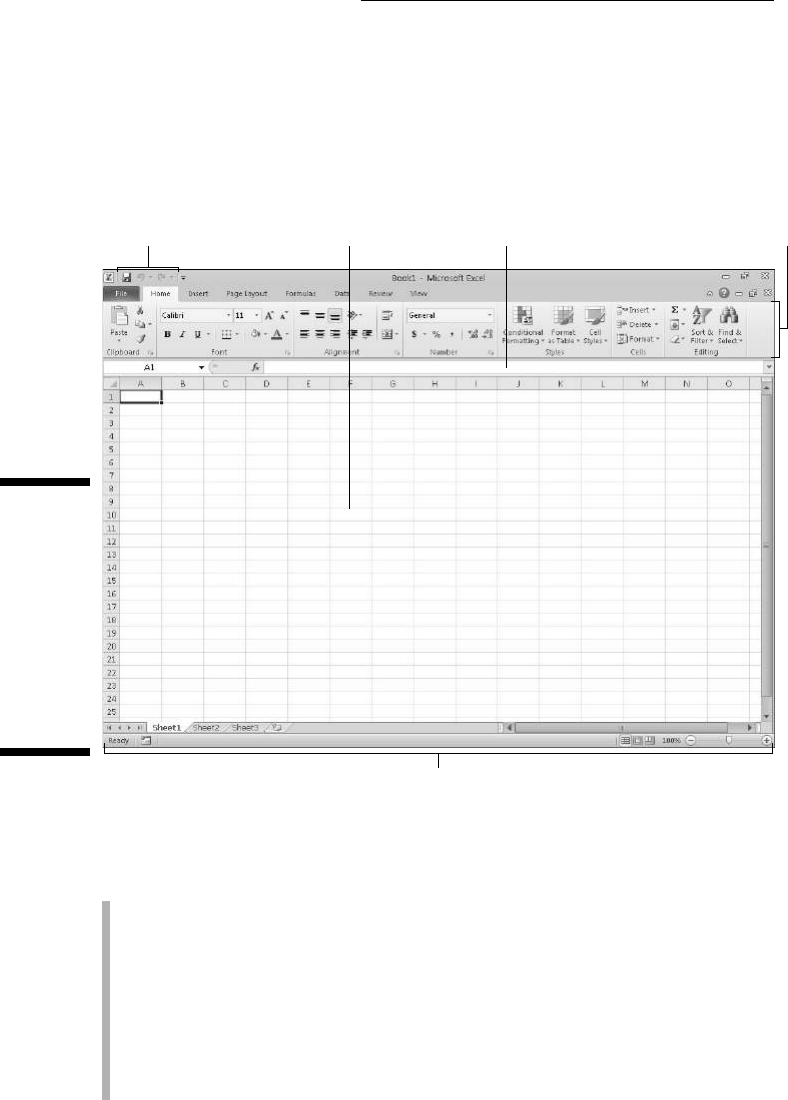
When you launch Excel 2010, the program opens the first of three new work-
sheets (named Sheet1) in a new workbook file (named Book1) inside a pro-
gram window like the one shown in Figure 1-1.
Figure 1-1:
The Excel
2010
program
window that
appears
immedi-
ately after
launching
the
program.
Quick Access toolbar Worksheet area Formula bar Ribbon
Status bar
The Excel program window containing this worksheet of the workbook con-
tains the following components:
✓ File tab that when clicked opens the new Backstage View — a menu
on the left that contains all the document- and file-related commands,
including Info (selected by default), Save, Save As, Open, Close, Recent,
New, Print, and Save & Send. Additionally, there’s a Help option with
add-ins, an Options item that enables you to change many of Excel’s
default settings, and an Exit option to quit the program.
✓ Customizable Quick Access toolbar that contains buttons you can click
to perform common tasks, such as saving your work and undoing and
redoing edits.
13
Chapter 1: The Excel 2010 User Experience
✓ Ribbon that contains the bulk of the Excel commands arranged into a
series of tabs ranging from Home through View.
✓ Formula bar that displays the address of the current cell along with the
contents of that cell.
✓ Worksheet area that contains the cells of the worksheet identified by
column headings using letters along the top and row headings using
numbers along the left edge; tabs for selecting new worksheets; a hori-
zontal scroll bar to move left and right through the sheet; and a vertical
scroll bar to move up and down through the sheet.
✓ Status bar that keeps you informed of the program’s current mode and
any special keys you engage, and enables you to select a new worksheet
view and to zoom in and out on the worksheet.
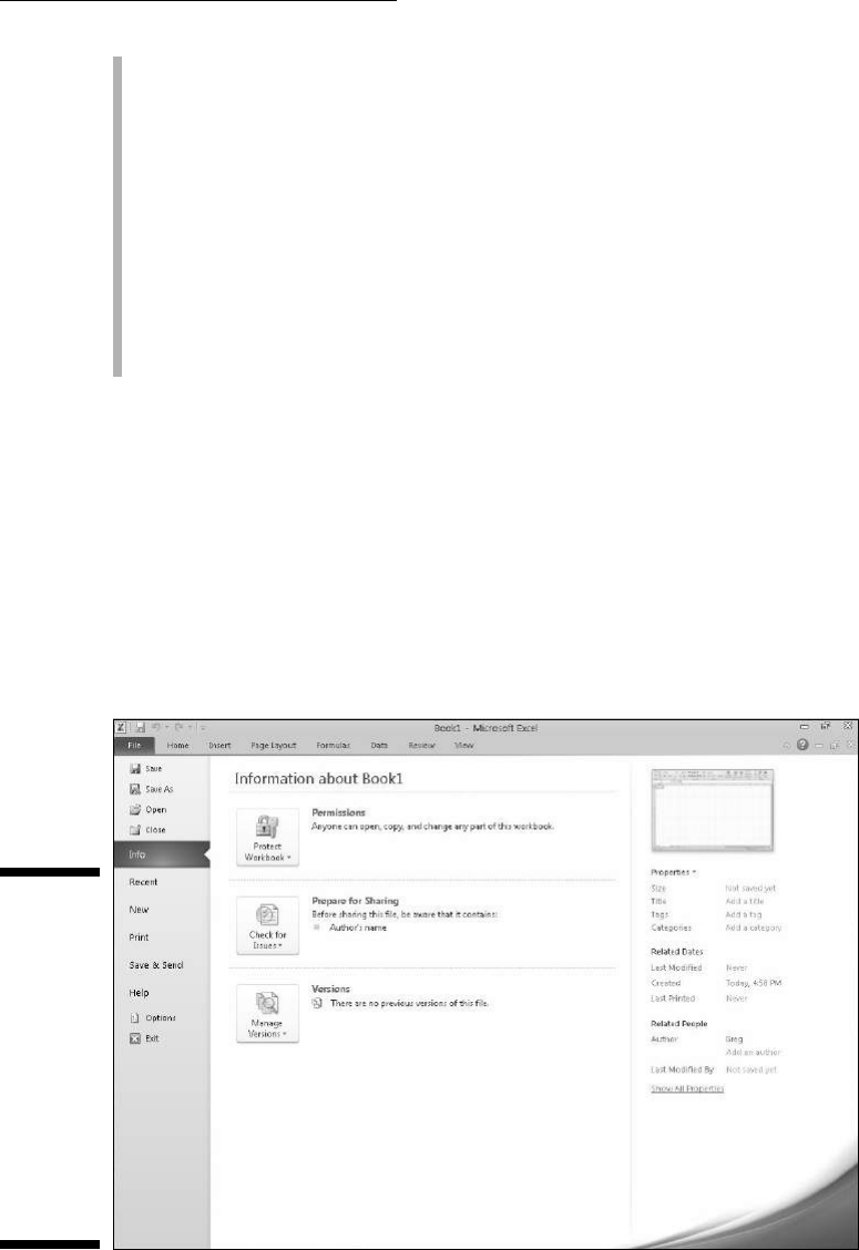
Going Backstage via File
To the immediate left of the Home tab on the Ribbon right below the Quick
Access toolbar, you find the File tab.
When you click File, the new Backstage View opens. This view contains a
menu similar to the one shown in Figure 1-2. When you open the Backstage
View, the Info option displays at-a-glance stats about the Excel workbook file
you have opened and active in the program.
Figure 1-2:
Open
Backstage
View to get
at-a-glance
information
about the
current file,
access all
file-related
commands,
and modify
the program
options.

14
Part I: Getting In on the Ground Floor
This information panel is divided into two panes. The pane on the left con-
tains large buttons that enable you to modify the workbook’s permissions,
distribution, and versions. The pane on the right contains a thumbnail of
the workbook followed by a list of fields detailing the workbook’s various
Document Properties, some of which you can change (such as Title, Tags,
Categories, and Author), and many of which you can’t (such as Size, Last
Modified, Created, and so forth).
Above the Info option, you find the commands (Save, Save As, Open, and
Close) you commonly need for working with Excel workbook files. Near the
bottom, the File tab contains a Help option that, when selected, displays a
Support panel in the Backstage View. This panel contains options for getting
help on using Excel, customizing its default settings, as well as checking for
updates to the Excel 2010 program. Below Help, you find options that you can
select to change the program’s settings, along with an Exit option that you
can select when you’re ready to close the program.
Click the Recent option to continue editing an Excel workbook you’ve worked
on of late. When you click the Recent option, Excel displays a panel with a list
of all the workbook files recently opened in the program. To re-open a particu-
lar file for editing, all you do is click its filename in this list.
To close the Backstage View and return to the normal worksheet view, you
can click the File tab a second time or simply press the Escape key.
Bragging about the Ribbon
The Ribbon (shown in Figure 1-3) changes the way you work in Excel 2010.
Instead of having to memorize (or guess) on which pull-down menu or tool-
bar Microsoft put the particular command you want to use, their designers
and engineers came up with the Ribbon that shows you the most commonly
used options needed to perform a particular Excel task.
Figure 1-3:
Excel’s
Ribbon
consists
of a series
of tabs
containing
command
buttons
arranged
into differ-
ent groups.
Tabs Dialog box launchers
Command buttons
Groups

15
Chapter 1: The Excel 2010 User Experience
The Ribbon contains the following components:
✓ Tabs for each of Excel’s main tasks that bring together and display all
the commands commonly needed to perform that core task.
✓ Groups that organize related command buttons into subtasks normally
performed as part of the tab’s larger core task.
✓ Command buttons within each group that you select to perform a par-
ticular action or to open a gallery from which you can click a particular
thumbnail. Note: Many command buttons on certain tabs of the Ribbon
are organized into mini-toolbars with related settings.
✓ Dialog box launcher in the lower-right corner of certain groups that
opens a dialog box containing a bunch of additional options you can
select.
To display more of the Worksheet area in the program window, you can mini-
mize the Ribbon so that only its tabs display. Simply click the Minimize the
Ribbon button, the first button with what looks like a greater than symbol
pointing upward in the group of buttons for minimizing, maximizing, and clos-
ing the current worksheet window to the right of the Ribbon tabs and to the
immediate left of the Help button. You can also double-click any one of the
Ribbon’s tabs, or just press Ctrl+F1. To redisplay the entire Ribbon, and keep
all the command buttons on its tabs displayed in the program window, click
the Expand the Ribbon button, double-click one of the tabs, or press Ctrl+F1 a
second time.
When you work in Excel with the Ribbon minimized, the Ribbon expands each
time you click one of its tabs to show its command buttons, but that tab stays
open only until you select one of the command buttons. The moment you
select a command button, Excel immediately minimizes the Ribbon again and
just displays its tabs.
Keeping tabs on the Excel Ribbon
The first time you launch Excel 2010, its Ribbon contains the following tabs
from left to right:
✓ Home tab with the command buttons normally used when creating, for-
matting, and editing a spreadsheet, arranged into the Clipboard, Font,
Alignment, Number, Styles, Cells, and Editing groups.
✓ Insert tab with the command buttons normally used when adding par-
ticular elements (including graphics, PivotTables, charts, hyperlinks,
and headers and footers) to a spreadsheet, arranged into the Tables,
Illustrations, Charts, Sparklines, Filter, Links, Text, and Symbols groups.
✓ Page Layout tab with the command buttons normally used when pre-
paring a spreadsheet for printing or re-ordering graphics on the sheet,
arranged into the Themes, Page Setup, Scale to Fit, Sheet Options, and
Arrange groups.

16
Part I: Getting In on the Ground Floor
✓ Formulas tab with the command buttons normally used when
adding formulas and functions to a spreadsheet or checking a worksheet
for formula errors, arranged into the Function Library, Defined Names,
Formula Auditing, and Calculation groups. Note: This tab also contains
a Solutions group when you activate certain add-in programs, such as
Analysis ToolPak and Euro Currency Tools. See Chapter 12 for more on
using Excel add-in programs.
✓ Data tab with the command buttons normally used when importing,
querying, outlining, and subtotaling the data placed into a worksheet’s
data list, arranged into the Get External Data, Connections, Sort & Filter,
Data Tools, and Outline groups. Note: This tab also contains an Analysis
group when you activate add-ins, such as Analysis ToolPak and Solver.
See Chapter 12 for more on Excel add-ins.
✓ Review tab with the command buttons normally used when proofing,
protecting, and marking up a spreadsheet for review by others, arranged
into the Proofing, Language, Comments, and Changes groups. Note:
This tab also contains an Ink group with a sole Start Inking button when
you’re running Office 2010 on a Tablet PC or a computer equipped with
a digital ink tablet.
✓ View tab with the command buttons normally used when changing the
display of the Worksheet area and the data it contains, arranged into the
Workbook Views, Show, Zoom, Window, and Macros groups.
In addition to these standard seven tabs, Excel has an eighth, optional
Developer tab that you can add to the Ribbon if you do a lot of work with
macros and XML files. See Chapter 12 for more on the Developer tab.
Although these standard tabs are the ones you always see on the Ribbon
when it displays in Excel, they aren’t the only things that can appear in this
area. Excel can display contextual tools when you’re working with a particu-
lar object that you select in the worksheet, such as a graphic image you’ve
added or a chart or PivotTable you’ve created. The name of the contextual
tools for the selected object appears immediately above the tab or tabs asso-
ciated with the tools.
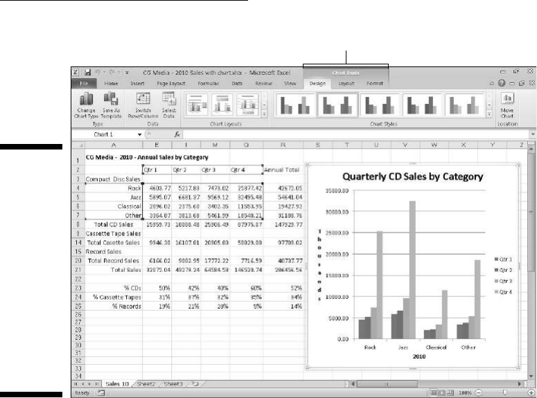
For example, Figure 1-4 shows a worksheet after you click the embedded
chart to select it. As you can see, doing this adds the contextual tool called
Chart Tools to the very end of the Ribbon. The Chart Tools contextual tool
has its own three tabs: Design (selected), Layout, and Format. Note, too, that
the command buttons on the Design tab are arranged into groups Type, Data,
Chart Layouts, Chart Styles, Location, and Mode.
The moment you deselect the object (usually by clicking somewhere outside
the object’s boundaries), the contextual tool for that object and all its tabs
immediately disappear from the Ribbon, leaving only the regular tabs —
Home, Insert, Page Layout, Formulas, Data, Review, and View — displayed.
17
Chapter 1: The Excel 2010 User Experience
Figure 1-4:
When you
select cer-
tain objects
in the
worksheet,
Excel adds
contextual
tools to
the Ribbon
with their
own tabs,
groups, and
command
buttons.
Chart Tools contextual tab
Selecting commands from the Ribbon
The most direct method for selecting commands on the Ribbon is to click the
tab that contains the command button you want and then click that button in
its group. For example, to insert a piece of clip art into your spreadsheet, you
click the Insert tab and then click the Clip Art button to open the Clip Art task
pane in the Worksheet area.
The easiest method for selecting commands on the Ribbon — if you know
your keyboard well — is to press the Alt key and then type the sequence of
letters designated as the hot keys for the desired tab and associated com-
mand buttons.
When you press and release the Alt key, Excel displays the hot keys for all
the tabs on the Ribbon. When you type one of the Ribbon tab hot keys to
select it, all the command button hot keys appear along with the hot keys
for the dialog box launchers (see Figure 1-5). To select a command button or
dialog box launcher, simply type its hot key letter(s).

18
Part I: Getting In on the Ground Floor
Figure 1-5:
Excel hot
keys for
selecting
command
buttons and
dialog box
launchers.
If you know the old Excel shortcut keys from versions Excel 97 through 2003,
you can still use them. For example, instead of going through the rigmarole
of pressing Alt+HC to copy a cell selection to the Office Clipboard and then
Alt+HV to paste it elsewhere in the sheet, you can still press Ctrl+C to copy
the selection and then press Ctrl+V when you’re ready to paste it. Note, how-
ever, that when using a hot key combination with the Alt key, you don’t need
to keep the Alt key depressed while typing the remaining letter(s) as you do
when using a shortcut key combo with the Ctrl key.
Customizing the Quick Access toolbar
When you start using Excel 2010, the Quick Access toolbar contains only the
following few buttons:
✓ Save to save any changes made to the current workbook using the same
filename, file format, and location
✓ Undo to undo the last editing, formatting, or layout change you made
✓ Redo to reapply the previous editing, formatting, or layout change that
you just removed with the Undo button
The Quick Access toolbar is very customizable because Excel makes it easy
to add any Ribbon command to it. Moreover, you’re not restricted to adding
buttons for just the commands on the Ribbon; you can add any Excel com-
mand you want to the toolbar, even the obscure ones that don’t rate an
appearance on any of its tabs.
By default, the Quick Access toolbar appears above the Ribbon tabs immedi-
ately to the right of the Excel program button (used to resize the workbook
window or quit the program). To display the toolbar beneath the Ribbon
immediately above the Formula bar, click the Customize Quick Access Toolbar
button (the drop-down button to the right of the toolbar with a horizontal bar

19
Chapter 1: The Excel 2010 User Experience
above a down-pointing triangle) and then click Show Below the Ribbon on
its drop-down menu. You will definitely want to make this change if you start
adding more buttons to the toolbar so that the growing Quick Access toolbar
doesn’t start crowding the name of the current workbook that appears to the
toolbar’s right.
Adding command buttons on the Customize
Quick Access Toolbar’s drop-down menu
When you click the Customize Quick Access Toolbar button, a drop-down
menu appears containing the following commands:
✓ New to open a new workbook
✓ Open to display the Open dialog box for opening an existing workbook
✓ Save to save changes to your current workbook
✓ E-mail to open your mail
✓ Quick Print to send the current worksheet to your default printer
✓ Print Preview to open the Print settings in Backstage View with a pre-
view of the current worksheet in the right pane
✓ Spelling to check the current worksheet for spelling errors
✓ Undo to undo your latest worksheet edit
✓ Redo to reapply the last edit that you removed with Undo
✓ Sort Ascending to sort the current cell selection or column in A to
Z alphabetical order, lowest to highest numerical order, or oldest to
newest date order
✓ Sort Descending to sort the current cell selection or column in Z to
A alphabetical order, highest to lowest numerical order, or newest to
oldest date order
When you open this menu, only the Save, Undo, and Redo options are
selected (indicated by the check marks); therefore, these buttons are the
only buttons to appear on the Quick Access toolbar. To add any of the other
commands on this menu to the toolbar, you simply click the option on the
drop-down menu. Excel then adds a button for that command to the end of
the Quick Access toolbar (and a check mark to its option on the drop-down
menu).
To remove a command button that you add to the Quick Access toolbar in
this manner, click the option a second time on the Customize Quick Access
Toolbar button’s drop-down menu. Excel removes its command button from
the toolbar and the check mark from its option on the drop-down menu.
20
Part I: Getting In on the Ground Floor
Adding command buttons on the Ribbon
To add a Ribbon command to the Quick Access toolbar, simply right-click its
command button on the Ribbon and then click Add to Quick Access Toolbar
on its shortcut menu. Excel then immediately adds the command button
to the very end of the Quick Access toolbar, immediately in front of the
Customize Quick Access Toolbar button.
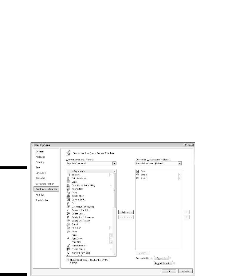
If you want to move the command button to a new location on the Quick
Access toolbar or group it with other buttons on the toolbar, click the
Customize Quick Access Toolbar button and then click the More Commands
option near the bottom of its drop-down menu.
Excel then opens the Excel Options dialog box with the Quick Access Toolbar
tab selected (similar to the one shown in Figure 1-6). On the right side of the
dialog box, Excel shows all the buttons added to the Quick Access toolbar.
The order in which they appear from left to right on the toolbar corresponds
to the top-down order in the list box.
Figure 1-6:
Use the
buttons on
the Quick
Access
Toolbar tab
of the Excel
Options
dialog box
to customize
the appear-
ance of
the Quick
Access
toolbar.
To reposition a particular button on the toolbar, click it in the list box
on the right and then click either the Move Up button (the one with the
black triangle pointing upward) or the Move Down button (the one with

21
Chapter 1: The Excel 2010 User Experience
the black triangle pointing downward) until the button is promoted or
demoted to the desired position on the toolbar.
You can add vertical separators to the toolbar to group related buttons. To do
this, click the <Separator> option in the list box on the left and then click the
Add button twice to add two. Then, click the Move Up or Move Down button
to position one of the two separators at the beginning of the group and the
other at the end.
To remove a button added from the Ribbon, right-click it on the Quick Access
toolbar and then click the Remove from Quick Access Toolbar option on its
shortcut menu.
Adding non-Ribbon commands to the Quick Access toolbar
You can also use the options on the Quick Access Toolbar tab of the Excel
Options dialog box (refer to Figure 1-6) to add a button for any Excel com-
mand even if it isn’t one of those displayed on the tabs of the Ribbon:
1. Click the type of command you want to add to the Quick Access tool-
bar in the Choose Commands From drop-down list box.
The types of commands include the Popular Commands pull-down menu
(the default) as well as each of the tabs that appear on the Ribbon. To
display only the commands that are not displayed on the Ribbon, click
Commands Not in the Ribbon near the top of the drop-down list. To
display a complete list of the Excel commands, click All Commands near
the top of the drop-down list.
2. Click the command whose button you want to add to the Quick Access
toolbar in the list box on the left.
3. Click the Add button to add the command button to the bottom of the
list box on the right.
4. (Optional) To reposition the newly added command button so that it
isn’t the last one on the toolbar, click the Move Up button until it’s in
the desired position.
5. Click the OK button to close the Excel Options dialog box.
If you’ve created favorite macros (see Chapter 12) that you routinely use and
want to be able to run directly from the Quick Access toolbar, click Macros in
the Choose Commands From drop-down list box in the Excel Options dialog
box and then click the name of the macro to add followed by the Add button.

22
Part I: Getting In on the Ground Floor
Having fun with the Formula bar
The Formula bar displays the cell address (determined by a column letter(s)
followed by a row number) and the contents of the current cell. For example,
cell A1 is the first cell of each worksheet at the intersection of column A and
row 1; cell XFD1048576 is the last cell of each worksheet at the intersection
of column XFD and row 1048576. The type of entry you make determines
the contents of the current cell: text or numbers, for example, if you enter
a heading or particular value, or the details of a formula if you enter a
calculation.
The Formula bar has three sections:
✓ Name box: The left-most section that displays the address of the current
cell address.
✓ Formula bar buttons: The second, middle section that appears as a
rather nondescript button displaying only an indented circle on the left
(used to narrow or widen the Name box) and the Insert Function button
(labeled fx) on the right. When you start making or editing a cell entry,
Cancel (an X) and Enter (a check mark) buttons appear between them.
✓ Cell contents: The third, right-most white area to the immediate right of
the Insert Function button takes up the rest of the bar and expands as
necessary to display really long cell entries that won’t fit in the normal
area.
The cell contents section of the Formula bar is important because it always
shows you the contents of the cell even when the worksheet does not. (When
you’re dealing with a formula, Excel displays only the calculated result in the
cell in the worksheet and not the formula by which that result is derived.)
Additionally, you can edit the contents of the cell in this area at anytime.
Similarly, when the cell contents area is blank, you know that the cell is empty
as well.
How you assign 26 letters to 16,384 columns
When it comes to labeling the 16,384 columns
of an Excel 2010 worksheet, our alphabet with
its measly 26 letters is simply not up to the task.
To make up the difference, Excel doubles the
letters in the cell’s column reference so that
column AA follows column Z (after which you
find column AB, AC, and so on) and then triples
them so that column AAA follows column ZZ
(after which you get column AAB, AAC, and the
like). At the end of this letter tripling, the 16,384th
and last column of the worksheet ends up being
XFD so that the last cell in the 1,048,576th row
has the cell address XFD1048576!

23
Chapter 1: The Excel 2010 User Experience
What to do in the Worksheet area
The Worksheet area is where most of the Excel spreadsheet action takes
place because it’s the place that displays the cells in different sections of the
current worksheet and it’s right inside the cells that you do all your spread-
sheet data entry and formatting, not to mention a great deal of your editing.
To enter or edit data in a cell, that cell must be current. Excel indicates that a
cell is current in three ways:
✓ The cell cursor — the dark black border surrounding the cell’s entire
perimeter — appears in the cell.
✓ The address of the cell appears in the Name box of the Formula bar.
✓ The cell’s column letter(s) and row number are shaded (in a kind of an
orange-beige color on most monitors) in the column headings and row
headings that appear at the top and left of the Worksheet area, respectively.
Moving around the worksheet
An Excel worksheet contains far too many columns and rows for all a work-
sheet’s cells to be displayed at one time regardless of how large your per-
sonal computer monitor screen is or how high the screen resolution. (After
all, we’re talking 17,179,869,184 cells total!) Therefore, Excel offers many
methods for moving the cell cursor around the worksheet to the cell where
you want to enter new data or edit existing data:
✓ Click the desired cell — assuming that the cell is displayed within the
section of the sheet visible in the Worksheet area.
Click the Name box, type the address of the desired cell, and then press
the Enter key.
✓ Press F5 to open the Go To dialog box, type the address of the desired
cell into its Reference text box, and then click OK.
✓ Use the cursor keys, as shown in Table 1-1, to move the cell cursor to
the desired cell.
✓ Use the horizontal and vertical scroll bars at the bottom and right edge
of the Worksheet area to move the part of the worksheet that contains
the desired cell and then click the cell to put the cell cursor in it.
Keystroke shortcuts for moving the cell cursor
Excel offers a wide variety of keystrokes for moving the cell cursor to a
new cell. When you use one of these keystrokes, the program automatically
scrolls a new part of the worksheet into view, if this is required to move the
cell pointer. In Table 1-1, I summarize these keystrokes, including how far
each one moves the cell pointer from its starting position.

24
Part I: Getting In on the Ground Floor
Table 1-1 Keystrokes for Moving the Cell Cursor
Keystroke Where the Cell Cursor Moves
→ or Tab
Cell to the immediate right.
← or Shift+Tab
Cell to the immediate left.
↑
Cell up one row.
↓
Cell down one row.
Home Cell in Column A of the current row.
Ctrl+Home First cell (A1) of the worksheet.
Ctrl+End or End, Home Cell in the worksheet at the intersection of the last
column that has data in it and the last row that has
data in it (that is, the last cell of the so-called active
area of the worksheet).
Page Up Cell one full screen up in the same column.
Page Down Cell one full screen down in the same column.
Ctrl+→ or End, →
First occupied cell to the right in the same row that is
either preceded or followed by a blank cell. If no cell
is occupied, the pointer goes to the cell at the very
end of the row.
Ctrl+← or End, ←
First occupied cell to the left in the same row that is
either preceded or followed by a blank cell. If no cell
is occupied, the pointer goes to the cell at the very
beginning of the row.
Ctrl+↑ or End, ↑
First occupied cell above in the same column that is
either preceded or followed by a blank cell. If no cell
is occupied, the pointer goes to the cell at the very
top of the column.
Ctrl+↓ or End, ↓
First occupied cell below in the same column that is
either preceded or followed by a blank cell. If no cell
is occupied, the pointer goes to the cell at the very
bottom of the column.
Ctrl+Page Down The cell pointer’s location in the next worksheet of
that workbook.
Ctrl+Page Up
The cell pointer’s location in the previous worksheet
of that workbook.
Note: In the case of those keystrokes that use arrow keys, you must either use the arrows on the cursor
keypad or else have the Num Lock disengaged on the numeric keypad of your keyboard.
The keystrokes that combine the Ctrl or End key with an arrow key listed in
Table 1-1 are among the most helpful for moving quickly from one edge to the
other in large tables of cell entries or for moving from table to table in a sec-
tion of a worksheet with many blocks of cells.

25
Chapter 1: The Excel 2010 User Experience
When you use Ctrl and an arrow key to move from edge to edge in a table or
between tables in a worksheet, you hold down Ctrl while you press one of the
four arrow keys (indicated by the + symbol in keystrokes, such as Ctrl+→).
When you use End and an arrow-key alternative, you must press and then
release the End key before you press the arrow key (indicated by the comma
in keystrokes, such as End, →). Pressing and releasing the End key causes the
End Mode indicator to appear on the status bar. This is your sign that Excel
is ready for you to press one of the four arrow keys.
Because you can keep the Ctrl key depressed while you press the different
arrow keys that you need to use, the Ctrl-plus-arrow-key method provides a
more fluid method for navigating blocks of cells than the End-then-arrow-key
method.
You can use the Scroll Lock key to “freeze” the position of the cell pointer in
the worksheet so that you can scroll new areas of the worksheet in view with
keystrokes, such as PgUp (Page Up) and PgDn (Page Down), without changing
the cell pointer’s original position. (In essence, making these keystrokes work
in the same manner as the scroll bars.)
After engaging Scroll Lock, when you scroll the worksheet with the keyboard,
Excel does not select a new cell while it brings a new section of the work-
sheet into view. To “unfreeze” the cell pointer when scrolling the worksheet
via the keyboard, you just press the Scroll Lock key again.
Tips on using the scroll bars
To understand how scrolling works in Excel, imagine its humongous work-
sheet as a papyrus scroll attached to rollers on the left and right. To bring
into view a section of papyrus hidden on the right, you crank the left roller
until the section with the cells that you want to see appears. Likewise, to
scroll into view a worksheet section hidden on the left, you crank the right
roller until the section of cells appears.
You can use the horizontal scroll bar at the bottom of the Worksheet area
to scroll back and forth through the columns of a worksheet and the verti-
cal scroll bar to scroll up and down through its rows. To scroll a column or
a row at a time in a particular direction, click the appropriate scroll arrow
at the ends of the scroll bar. To jump immediately back to the originally dis-
played area of the worksheet after scrolling through single columns or rows
in this fashion, simply click the area in the scroll bar that now appears in
front of or after the scroll bar.
You can resize the horizontal scroll bar making it wider or narrower by drag-
ging the button that appears to the immediate left of its left scroll arrow. Just
keep in mind when working in a workbook that contains a whole bunch of
worksheets that widening the horizontal scroll bar can hide the display of the
workbook’s later sheet tabs.

26
Part I: Getting In on the Ground Floor
To scroll very quickly through columns or rows of the worksheet, hold down
the Shift key and then drag the scroll button in the appropriate direction
within the scroll bar until the columns or rows that you want to see appear on
the screen in the Worksheet area. When you hold down the Shift key while you
scroll, the scroll button within the scroll bar becomes skinny and a ScreenTip
appears next to the scroll bar, keeping you informed of the letter(s) of the col-
umns or the numbers of the rows that you’re whizzing through.
If your mouse has a wheel, you can use it to scroll directly through the
columns and rows of the worksheet without using the horizontal or verti-
cal scroll bars. Simply position the white cross mouse pointer in the center
of the Worksheet area and then hold down the wheel button of the mouse.
When the mouse pointer changes to a four-pointed arrow with a black dot in
its center, drag the mouse pointer in the appropriate direction (left and right
to scroll through columns or up and down to scroll through rows) until the
desired column or row comes into view in the Worksheet area.
The only disadvantage to using the scroll bars to move around is that the
scroll bars bring only new sections of the worksheet into view — they don’t
actually change the position of the cell cursor. If you want to start making
entries in the cells in a new area of the worksheet, you still have to remember
to select the cell (by clicking it) or the group of cells (by dragging through
them) where you want the data to appear before you begin entering the data.
Surfing the sheets in a workbook
Each new workbook you open in Excel 2010 contains three blank worksheets,
each with its own 16,384 columns and 1,048,576 rows (giving you a truly stag-
gering 51,539,607,552 blank cells!). But, that’s not all. If ever you need more
worksheets in your workbook, you can add them simply by clicking the Insert
Worksheet button that appears to the immediate right of the last sheet tab
(see Figure 1-7) or by pressing Shift+F11.
Figure 1-7:
The Sheet
Tab scroll
buttons,
sheet tabs,
and Insert
Worksheet
button
enable you
to activate
your work-
sheets and
add to them.
First sheet
Previous sheet
Next sheet
Last sheet
Current sheet
Sheet Tab
scroll buttons
Insert worksheet

27
Chapter 1: The Excel 2010 User Experience
On the left side of the bottom of the Worksheet area, the Sheet Tab scroll but-
tons appear followed by the actual tabs for the worksheets in your workbook
and the Insert Worksheet button. To activate a worksheet for editing, you
select it by clicking its sheet tab. Excel lets you know what sheet is active by
displaying the sheet name in boldface type and making its tab appear on top
of the others.
Don’t forget the Ctrl+Page Down and Ctrl+Page Up shortcut keys for selecting
the next and previous sheet, respectively, in your workbook.
If your workbook contains too many sheets for all the tabs to display at the
bottom of the Worksheet area, use the Sheet Tab scroll buttons to bring new
tabs into view (so that you can then click them to activate them). You click
the Next Sheet button to scroll the next hidden sheet tab into view or the
Last Sheet button to scroll the last group of completely or partially hidden
tabs into view.
Showing off the Status bar
The Status bar is the last component at the very bottom of the Excel program
window (see Figure 1-8). The Status bar contains the following:
✓ Mode indicator that shows the current state of the Excel program
(Ready, Edit, and so on) as well as any special keys that are engaged
(Caps Lock, Num Lock, and Scroll Lock).
✓ AutoCalculate indicator that displays the average and sum of all the
numerical entries in the current cell selection along with the count of
every cell in the selection.
One reason for adding extra sheets to a workbook
You may wonder why anyone would ever need
more than three worksheets given just how
many cells each individual sheet contains.
The truth is that it’s all about how you choose
to structure a particular spreadsheet rather
than running out of places to put the data. For
example, suppose that you need to create a
workbook that contains budgets for all the
various departments in your corporation, you
may decide to devote an individual worksheet
to each department (with the actual budget
spreadsheet tables laid out in the same manner
on each sheet) rather than placing all the tables
in different sections of the same sheet. Using
this kind of one-sheet-per-budget layout makes
it much easier for you to find each budget, print
each one as a separate page of a report, and,
if ever necessary, to consolidate the data in a
separate summary worksheet.

28
Part I: Getting In on the Ground Floor
✓ Layout selector that enables you to select between three layouts for the
Worksheet area: Normal, the default view that shows only the worksheet
cells with the column and row headings; Page Layout View that adds
rulers, page margins, and shows page breaks for the worksheet; and
Page Break Preview that enables you to adjust the paging of a report.
(See Chapter 5 for details.)
✓ Zoom slider that enables you to zoom in and out on the cells in the
Worksheet area by dragging the slider to the right or left, respectively.
Figure 1-8:
The Status
bar dis-
plays the
program’s
current
standing
and enables
you to
select new
worksheet
views.
Layout selector
Mode indicator Auto Calculate indicator Zoom slider
The Num Lock indicator tells you that you can use the numbers on the numeric
keypad for entering values in the worksheet. This keypad will most often be
separate from the regular keyboard (on the right side if you’re using a separate
keyboard) and embedded in keys on the right side of the keyboard on almost all
laptop computers where the keyboard is built in to the computer.
Launching and Quitting Excel
Excel 2010 runs under both the older Windows XP operating system and the
newer Vista and Windows 7 operating systems. Because of changes made to
the Start menu in Windows Vista and Windows 7, the procedure for starting
Excel from these versions of Windows is a bit different from Windows XP.
Starting Excel from the Start menu
You can use the Start Search box at the bottom of the Windows Vista Start
menu or the Search Programs and Files search box on the Windows 7

29
Chapter 1: The Excel 2010 User Experience
Start menu to locate Excel on your computer and launch the program in no
time at all:
1. Click the Start button on the Windows taskbar to open the Windows
Start menu.
2. Click the Start menu’s search text box and type the letters exc to have
Windows locate Microsoft Office Excel 2010 on your computer.
3. Click the Microsoft Excel 2010 option that now appears in the left
Programs column on the Start menu.
If you have more time on your hands, you can also launch Excel from the
Windows Start menu by going through the rigmarole of clicking Start➪All
Programs➪Microsoft Office➪Microsoft Excel 2010.
Starting Excel from the Windows
XP Start menu
When starting Excel 2010 from the Windows XP Start menu, you follow these
simple steps:
1. Click the Start button on the Windows taskbar to open the Windows
Start menu.
2. With the mouse, highlight All Programs on the Start menu and then
Microsoft Office on the Start continuation menu before clicking the
Microsoft Excel 2010 option on the Microsoft Office continuation
menu.
Pinning a Microsoft Excel 2010 option
on your Windows Start menu
If you use Excel all the time, you may want to make its program option a
permanent part of the Windows Start menu. To do this, you pin the pro-
gram option to the Start menu (and the steps for doing this are the same in
Windows XP as they are in Windows Vista and Windows 7):
1. Click the Windows Start button and then highlight the All Programs
option on the Start menu.
Windows XP opens a continuation menu from its Start menu and
Windows Vista and Windows 7 display a new menu of program options
on their Start menus.

30
Part I: Getting In on the Ground Floor
2. Highlight the Microsoft Office option on the Windows XP continua-
tion menu or click the Microsoft Office option on the Windows Vista/7
Start menu.
Windows XP displays a continuation menu with a list of all the Office
2010 programs installed on your computer. Windows Vista and Windows 7
display a submenu listing the Office 2010 programs.
3. Right-click Microsoft Excel 2010 on the Windows continuation or sub-
menu to open its shortcut menu.
4. Click Pin to Start Menu on the shortcut menu.
After pinning Excel in this manner, the Microsoft Excel 2010 option always
appears in the upper section of the left-hand column of the Windows Start
menu and you can then launch Excel simply by clicking the Windows Start
button and then clicking this menu option.
After you pin the Microsoft Excel 2010 option on to the Windows 7 Start menu,
whenever you highlight this menu item, Windows 7 automatically expands
the Start menu to display a list of your recently opened Excel workbook files.
You can then open one of these files for further editing at the same time you
launch the Excel 2010 program by clicking its filename on the Start menu.
Adding a Microsoft Excel 2010 shortcut
to your Windows desktop
Some people prefer having the Excel program icon appear on the Windows
desktop so that they can launch the program from the desktop by double-
clicking this program icon. To create a Microsoft Excel 2010 program short-
cut for your Windows desktop, you follow these steps:
1. Click the Windows Start button and then highlight the All Programs
option on the Start menu.
Windows XP opens a continuation menu from its Start menu and
Windows Vista and Windows 7 display a new menu of program options
on their Start menus.
2. Highlight the Microsoft Office option on the Windows XP continua-
tion menu or click the Microsoft Office option on the Windows Vista/
Windows 7 Start menu.
Windows XP displays a continuation menu with a list of all the Office
2010 programs installed on your computer. Windows Vista and Windows 7
display a submenu listing the Office 2010 programs.

31
Chapter 1: The Excel 2010 User Experience
3. Right-click Microsoft Excel 2010 on the Windows continuation or sub-
menu to open its shortcut menu.
4. Highlight the Send To option on this menu and then click Desktop
(Create Shortcut) on the continuation shortcut menu.
Windows adds a Microsoft Excel 2010 shortcut icon to your Windows
desktop that launches the program when you double-click it or right-
click it and then click the Open option.
Adding Excel to the Windows
Quick Launch toolbar
If you want to be able to launch Excel 2010 by clicking a single button, drag
the Excel icon for your Windows Vista or Windows XP desktop shortcut to
the Quick Launch toolbar to the immediate right of the Start button at the
beginning of the Windows taskbar. When you position the icon on this tool-
bar, Windows indicates where the new Excel button will appear by drawing
a black, vertical I-beam in front of or between the existing buttons on this
bar. As soon as you release the mouse button, Windows adds an Excel 2010
button to the Quick Launch toolbar that enables you to launch the program
by a single click of its icon.
Pinning an Excel icon to the
Windows 7 taskbar
If your computer is running Windows 7, you can add a Microsoft Excel 2010
icon to the taskbar in addition to the standard Internet Explorer, Windows
Explorer, and Windows Media Player buttons.
All you do is drag and drop the Microsoft Excel 2010 icon that either you
pinned to the Windows Start menu or you added as a shortcut to the
Windows desktop into its desired position on the Windows 7 taskbar. (See
“Pinning a Microsoft Excel 2010 option on your Windows Start menu” and
“Adding a Microsoft Excel 2010 shortcut to your Windows desktop” earlier in
this chapter for details.)
After pinning a Microsoft Excel 2010 icon to the Windows 7 taskbar, the button
appears on the Windows taskbar each time you start your computer, and you
can launch the Excel program simply by single clicking its icon.

32
Part I: Getting In on the Ground Floor
Exiting Excel
When you’re ready to call it a day and quit Excel, you have several choices
for shutting down the program:
✓ Choose File➪Exit.
✓ Press Alt+FX or Alt+F4.
✓ Click the Close button (the X) in the upper-right corner of the Excel pro-
gram window.
If you try to exit Excel after working on a workbook and you haven’t saved
your latest changes, the program displays an alert box querying whether
you want to save your changes. To save your changes before exiting, click
the Save command button. (For detailed information on saving documents,
see Chapter 2.) If you’ve just been playing around in the worksheet and don’t
want to save your changes, you can abandon the document by clicking the
Don’t Save button.
Help Is on the Way
You can get online help with Excel 2010 anytime that you need it while using
the program. Simply click the Help button (the button with the question mark
icon to the immediate right of the Minimize the Ribbon button on the right
side of the program window opposite the Ribbon’s tabs) or press F1 to open
a separate Excel Help window. (See Figure 1-9.)
When the Excel Help window opens, Excel attempts to use your Internet con-
nection to update its topics. The opening Help window contains links that
you can click to get information on what’s new in the program.
To get help with a particular command or function, use the Search text box
at the top of the Excel Help window. Type keywords or a phrase describing
your topic (such as “print preview” or “printing worksheets”) in this text box
and then press Enter or click the Search button. The Excel Help window then
presents a list of links to related help topics that you can click to display the
information.
To print the help topic displayed in the Excel Help window, click the Print
button (with the printer icon) on its toolbar. Excel then opens a Print dialog
box where you can select the printer and options to use in printing the
information.
To display a table of contents with all the main categories and subtopics
arranged hierarchically, click the Show Table of Contents button (with the
book icon) on the toolbar.
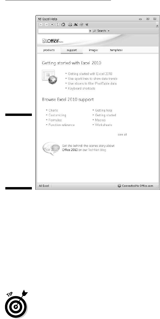
33
Chapter 1: The Excel 2010 User Experience
Figure 1-9:
The Excel
Help
window
automatically
connects
you to the
Internet
when you
open it.
Migrating to Excel 2010 from Earlier
Versions Using Pull-down Menus
If you’re a brand new Excel user or have had some experience with Excel
2007, you’re going to take to Excel 2010’s Ribbon User Interface like a duck to
water. However, if you’re coming to Excel 2010 as a dedicated user of earlier
Excel versions (Excel 97 all the way through Excel 2003), the first time you
launch Excel 2010 and take a gander at the Ribbon, you’re probably going to
feel more like someone just threw you into the deep end of the pool without a
life preserver.
Don’t panic! Simply use this section of the chapter as your Excel 2010 life
preserver. It’s intended to get you oriented, keep your head above water, and
have you swimming with the new interface in no time at all. Just give me five
minutes of your precious time and I promise I’ll have you up and running with
Excel 2010 and maybe even smiling again. Now, take a deep breath, and here
we go. . . .

34
Part I: Getting In on the Ground Floor
First, the bad news: There is no Classic mode in Excel 2010 that will magically
turn that fat, screen real estate–stealing Ribbon back into those sleek, tried
and true pull-down menus (thanks Microsoft, I needed that!). After the won-
derful designers and engineers at Microsoft got through dumping all the pull-
down menus and toolbars that you worked so diligently to master and on
which you relied every Excel workday of your life, there was just nothing left
for them to hang a Classic mode onto.
Now, for the good news: You really don’t need a Classic mode — you just
need to find out where those scoundrel engineers went and put all the stuff
you used to do so effortlessly in versions of Excel before the Ribbon User
Interface. After all, you already know what most of those pull-down menu
items and toolbar buttons do; all you have to do is locate them.
Cutting the Ribbon down to size
Want to get that busy Ribbon out of your face? At this point, it’s just taking
up valuable space and probably making you crazy. So, please double-click
any one of the tabs or press Ctrl+F1 right now to cut the Ribbon display down
to only its tabs. Single-clicking a tab then temporarily redisplays the Ribbon
until you select one of its command buttons, whereas pressing Ctrl+F1 a
second time redisplays the Ribbon and keeps it open in all its glory.
When only the tabs — Home through View — are showing at the top of
the Excel program window, you should feel a whole lot more comfortable
with the screen. The Excel 2010 screen is then as clean and uncluttered, if
not more, as the earlier version of Excel that you were using with only the
Quick Access toolbar, Ribbon tabs, and Formula bar displayed above the
Worksheet area.
Now, you’re probably wondering where those Microsoft engineers moved the
most important and commonly used pull-down menu commands. Table 1-2
shows the Excel 2010 equivalents for the menu commands you probably used
most often in doing your work in the earlier version of Excel.
When a particular command is assigned to one of the tabs on the Ribbon,
Table 1-2 lists only the tab and command button name without naming the
group because the group name plays no part in selecting the command.
For example, the table lists the View➪Header and Footer command as
Insert➪Header & Footer without regard to the fact that the Header & Footer
button is part of the Text group on the Insert tab.

35
Chapter 1: The Excel 2010 User Experience
Table 1-2 Excel 2010 Equivalents for Common
Pull-down Menu Commands in Excel 2003
Excel 2003 Command Excel 2010 Equivalent Common
Shortcut
Keys
Excel 2010
Shortcut
Keys
File Menu
File➪New File➪New Ctrl+N Alt+FN
File➪Open File➪Open Ctrl+O Alt+FO
File➪Save File➪Save or Save button
on the Quick Access
toolbar
Ctrl+S Alt+FS
File➪Save As File➪Save As F12 Alt+FA
File➪Print File➪Print Ctrl+P Alt+FP
File➪Send To➪Mail
Recipient
File➪Share➪
Send Using Email
Alt+FHE
File➪Send To➪
Recipient Using
Internet Fax Service
File➪Share➪
Send as Internet Fax
Alt+FHIF
File➪Close File➪Close Ctrl+W Alt+FC
Edit Menu
Edit➪Office Clipboard Home➪Clipboard group’s
dialog box launcher
Alt+HFO
Edit➪Clear➪All Home➪Clear (eraser
icon)➪Clear All
Alt+HEA
Edit➪Clear➪Formats Home➪Clear (eraser
icon)➪Clear Formats
Alt+HEF
Edit➪Clear➪Contents Home➪Clear (eraser
icon) ➪Clear Contents
Delete
key
Alt+HEC
Edit➪Clear➪Comments Home➪Clear (eraser
icon) ➪Clear Comments
Alt+HEM
Edit➪Delete Home➪Delete Alt+HD
Edit➪Move or Copy Sheet Home➪Format➪Move or
Copy Sheet
Alt+HOM
Edit➪Find Home➪Find & Select➪
Find
Ctrl+F Alt+HFDF
Edit➪Replace Home➪Find & Select➪
Replace
Ctrl+H Alt+HFDR
(continued)

36
Part I: Getting In on the Ground Floor
Table 1-2 (continued)
Excel 2003 Command Excel 2010 Equivalent Common
Shortcut
Keys
Excel 2010
Shortcut
Keys
View Menu
View➪Header and Footer Insert➪Header & Footer Alt+NH
View➪Full Screen View➪Full Screen Alt+WE
Insert Menu
Insert➪Cells Home➪Insert➪
Insert Cells
Alt+HII
Insert➪Rows Home➪Insert➪
Insert Sheet Rows
Alt+HIR
Insert➪Columns Home➪Insert➪
Insert Sheet Columns
Alt+HIC
Insert➪Worksheets Home➪Insert➪Insert
Sheet
Alt+HIS
Insert➪Symbol Insert➪Symbol Alt+NU
Insert➪Page Break Page Layout➪Breaks➪
Insert Page Break
Alt+PBI
Insert➪Name➪
Define
Formulas➪Define
Name➪Define Name
Alt+MMD
Insert➪Name➪
Paste
Formulas➪Use in Formula Alt+MS
Insert➪Name➪
Create
Formulas➪Create from
Selection
Alt+MC
Insert➪Name➪Label Formulas➪Name Manager Alt+MN
Insert➪Comment Review➪New Comment Alt+RC
Insert➪Picture Insert➪Picture Alt+NP
Insert➪Hyperlink Insert➪Hyperlink Ctrl+K Alt+NI
Format Menu
Format➪Cells Home➪Format➪
Format Cells
Ctrl+1 Alt+HOE
Format➪Row➪
Height
Home➪Format➪
Row Height
Alt+HOH
Format➪Row➪
AutoFit
Home➪Format➪
AutoFit Row Height
Alt+HOA

37
Chapter 1: The Excel 2010 User Experience
Excel 2003 Command Excel 2010 Equivalent Common
Shortcut
Keys
Excel 2010
Shortcut
Keys
Format➪Row➪
Hide/Unhide
Home➪Format➪Hide
& Unhide➪Hide Rows/
Unhide Rows
Alt+HOUR/
Alt+HOUO
Format➪Column➪
Width
Home➪Format➪Column
Width
Alt+HOW
Format➪Column➪Hide/
Unhide
Home➪Format➪Hide &
Unhide➪Hide Columns/
Unhide Columns
Alt+HOUC/
Alt+HOUL
Format➪Column➪
Standard Width
Home➪Format➪
Default Width
Alt+HOD
Format➪Sheet➪Rename Home➪Format➪
Rename Sheet
Alt+HOR
Format➪Sheet➪Hide/
Unhide
Home➪Format➪
Hide & Unhide➪
Hide Sheet/Unhide Sheet
Alt+HOUS/
Alt+HOUH
Format➪Sheet➪
Background
Page Layout➪Background Alt+PG
Format➪Sheet➪
Tab Color
Home➪Format➪Tab Color Alt+HOT
Format➪AutoFormat Home➪Format as Table Alt+HT
Format➪Conditional
Formatting
Home➪Conditional
Formatting
Alt+HL
Format➪Style Home➪Cell Styles Alt+HJ
Tools Menu
Tools➪Spelling Review➪Spelling F7 Alt+RS
Tools➪Research Review➪Research Alt+RR
Tools➪Error Checking Formulas➪Error Checking Alt+MK
Tools➪Speech➪
Show Text to Speech
Toolbar
Available only as custom
Speak Cells, Speak Cells -
Stop Speaking Cells,
Speak Cells by Columns,
Speak Cells by Rows,
and Speak Cells on Enter
buttons added to Quick
Access toolbar
(continued)

38
Part I: Getting In on the Ground Floor
Table 1-2 (continued)
Excel 2003 Command Excel 2010 Equivalent Common
Shortcut
Keys
Excel 2010
Shortcut
Keys
Tools➪Track Changes Review➪Track Changes Alt+RG
Tools➪Protection➪
Protect Sheet
Review➪Protect Sheet Alt+RPS
Tools➪Protection➪Allow
Users to Edit Ranges
Review➪Allow Users to
Edit Ranges
Alt+RU
Tools➪Protection➪
Protect Workbook
Review➪Protect
Workbook
Alt+RPW
Tools➪Protection➪
Protect and Share
Workbook
Review➪
Protect and Share
Workbook
Alt+RO
Tools➪Macro View➪Macros Alt+F8 Alt+WMV
Tools➪Add-Ins File➪Options➪Add-Ins Alt+FIAA
and then
Alt+G
Tools➪
AutoCorrect Options
File➪Options➪Proofing➪
AutoCorrect Options
Alt+FIP
and then
Alt+A
Tools➪Options File➪Options Alt+FI
Data Menu
Data➪Sort Home➪Sort & Filter➪
Custom Sort
Alt+HSU
Data➪Filter➪
AutoFilter
Data➪Filter Alt+AT
Data➪Filter➪
Advanced Filter
Data➪Advanced Alt+AQ
Data➪Form Available only as a custom
Form button added to
Quick Access toolbar
Data➪Subtotals Data➪Subtotal Alt+AB
Data➪Validation Data➪Data Validation➪
Data Validation
Alt+AVV
Data➪Table Data➪What-If Analysis➪
Data Table
Alt+AWT

39
Chapter 1: The Excel 2010 User Experience
Excel 2003 Command Excel 2010 Equivalent Common
Shortcut
Keys
Excel 2010
Shortcut
Keys
Data➪Text to
Columns
Data➪Text to Columns Alt+AE
Data➪
Consolidate
Data➪Consolidate Alt+AN
Data➪
Group and Outline
Data➪Group/Ungroup Alt+AG/
Alt+AU
Data➪PivotTable and
PivotChart Report
Insert➪PivotTable➪
PivotTable/PivotChart
Alt+NVT/
Alt+NVC
Data➪Import External
Data
Data➪From Other Sources Alt+AFO
Window Menu
Window➪New Window View➪New Window Alt+WN
Window➪Arrange View➪Arrange All Alt+WA
Window➪Compare Side
by Side
View➪View Side by Side
(two-page icon in Window
group)
Alt+WB
Window➪Hide, Unhide View➪Hide/Unhide Alt+WH/
Alt+WU
Window➪Split View➪Split Alt+WS
Window➪Freeze Panes View➪Freeze Panes Alt+WF
For the most part, the pull-down menu commands listed in Table 1-2 are logi-
cally located. The ones that take the most getting used to are the Header &
Footer and PivotTable/Chart commands that are located on the Insert tab
rather than the View tab and Data tab as might be expected given they inhab-
ited, respectively, the View and Data pull-down menus in earlier Excel ver-
sions. Additionally, the worksheet background command ended up all by its
lonesome on the Page Layout tab rather than going to the Home tab with all
its fellow formatting commands.
Finding the Standard toolbar
buttons equivalents
If you’re like me, you came to rely heavily on the buttons of the Standard
toolbar in doing all sorts of everyday tasks in earlier versions of Excel. Table

40
Part I: Getting In on the Ground Floor
1-3 shows you the Excel 2010 equivalents for the buttons on the Standard
toolbar in Excel 2003. As you can see from this table, most of the Standard
toolbar buttons are regulated to one of these places in Excel 2010:
✓ Backstage View activated by clicking the File tab or pressing Alt+F (New,
Open, Save, Print)
✓ Quick Access toolbar (Save, Undo, and Redo)
✓ Home tab in the Clipboard group (Cut, Copy, Paste, and Format Painter)
and Editing group (AutoSum, Sort Ascending, and Sort Descending)
Table 1-3 Excel 2010 Equivalents for the
Standard Toolbar Buttons in Excel 2003
Toolbar
Button
Excel 2010 Equivalent Common
Shortcut Keys
Excel 2010
Shortcut Keys
New File➪New Ctrl+N Alt+FN
Open File➪Open Ctrl+O Alt+FO
Save File➪Save or Save
button on Quick
Access toolbar
Ctrl+S Alt+FS
Permission Available only as a
custom Permission
button added to Quick
Access toolbar
E-mail File➪Share➪Send
Using E-mail
Alt+FHE
Print Quick Print button on
Quick Access toolbar
Print
Preview
File➪Print Alt+FP
Spelling Review➪Spelling F7 Alt+RS
Research Review➪Research Alt+RR
Cut Home➪Cut (scissors
icon in Clipboard
group)
Ctrl+X Alt+HX
Copy Home➪Copy
(double-sheet icon in
Clipboard group)
Ctrl+C Alt+HC
Paste Home➪Paste Ctrl+V Alt+HV

41
Chapter 1: The Excel 2010 User Experience
Toolbar
Button
Excel 2010 Equivalent Common
Shortcut Keys
Excel 2010
Shortcut Keys
Format
Painter
Home➪Format
Painter (brush icon in
Clipboard group)
Alt+HFP
Undo Undo button on Quick
Access toolbar
Ctrl+Z
Redo Redo button on Quick
Access toolbar
Ctrl+Y
Insert Ink
Annotations
Review➪Start Inking
(appears only on
Tablet PCs or comput-
ers with a digital ink
tablet)
Alt+RK
Insert
Hyperlink
Insert➪Hyperlink Ctrl+K Alt+NI
AutoSum Home➪AutoSum
(∑ - Sigma icon)
Alt+HU
Sort
Ascending
Home➪Sort &
Filter➪Sort A to Z
Alt+HSS
Sort
Descending
Home➪Sort &
Filter➪Sort Z to A
Alt+HSO
Chart Wizard Not available except
as specific chart type
command buttons in
the Charts group on
the Insert tab
Drawing Not available except
as command buttons
in the Illustrations
and Text groups on
the Insert tab, and as
custom buttons added
to Quick Access
toolbar
Zoom View➪Zoom Alt+WQ
Microsoft
Excel Help
Microsoft Office Excel
Help button to the
right of the Ribbon
tabs
F1

42
Part I: Getting In on the Ground Floor
Because Excel 2010 supports only a single toolbar (the Quick Access toolbar),
the Drawing toolbar disappears completely from Excel 2010, thus the Drawing
button on the Standard toolbar has no equivalent. Most of its main features,
including clip art, inserting graphics files, and creating diagrams and WordArt
are now on the Insert tab. Also, Excel 2010 doesn’t have an equivalent to the
Chart Wizard button on the Standard toolbar because you can create a chart
in a split-second by clicking the Column, Line, Pie, Bar, Area, Scatter, or Other
Charts command buttons on the Insert tab (see Chapter 10).
Finding the Formatting toolbar
buttons equivalents
Finding the Excel 2010 equivalents for the buttons on the Formatting toolbar
in earlier versions of Excel couldn’t be easier: Every one of the buttons on the
Formatting toolbar is displayed prominently on the Home tab of the Ribbon.
They’re all easy to identify because they use the same icons as before and
are located in the Font, Alignment, or Number group on the Home tab (refer
to Figure 1-3).
In addition to the Font, Font Size, Bold, Italic, Underline, Borders, Fill Color,
and Font Color buttons from the Formatting toolbar, the Font group also con-
tains the following two buttons:
✓ Increase Font Size button that bumps up the current font size a point
✓ Decrease Font Size button that reduces the current font size by a point
In addition to the Left Align, Center, Right Align, Decrease Indent, Increase
Indent, and Merge & Center buttons, the Alignment group also contains the
following buttons:
✓ Top Align button that vertically aligns the data entered into the current
cell selection with the top edge of the cell
✓ Middle Align button that vertically centers the data entered into the
current cell selection
✓ Bottom Align button that aligns the data entered in the current cell
selection with the bottom edge of the cell
✓ Orientation button that opens a pop-menu of orientation options that
enable you to change the direction of the text entered into the current
cell selection (by angling it up or down, converting it to vertical text, or
rotating it up or down) and open the Alignment tab of the Format Cells
dialog box
✓ Wrap Text button that applies wrap text to the current cell selection so
that Excel expands the row heights as needed to fit all its text within the
current column widths

43
Chapter 1: The Excel 2010 User Experience
In addition to the Percent Style, Comma Style, Increase Decimal, and
Decrease Decimal buttons from the Formatting toolbar, the Numbers group
contains the following buttons:
✓ Accounting Number Format button that enables you to select among
several different currency formats from U.S. dollars to Swiss Francs, as
well as to open the Number tab of the Format Cells dialog box with the
Accounting number format selected
✓ Number Format button that opens a pop-up menu of different number
options from General through Text, as well as opens the Number tab in the
Format Cells dialog box when you select its More Number Formats option
Putting the Excel Quick Access toolbar
to good use during the transition
Figure 1-10 shows you the Excel 2010 program window with the Ribbon mini-
mized and a completely customized Quick Access toolbar moved down so that
it appears under the tabs and above the Formula bar. This completely custom
version of the Quick Access toolbar should seem very familiar to you: It con-
tains every button from the Standard and Formatting toolbar in Excel 2003
with the exception of the Permission, Drawing, Zoom, and Help buttons. The
Permission button is so esoteric and seldom used that I didn’t bother to add
it. The Drawing button has no equivalent in Excel 2010. And neither the Zoom
button nor the Help button is really needed because the Zoom slider that
enables you to quickly select a new screen magnification percentage always
displays in the lower-right corner of the Excel 2010 Status bar and the Help
button always displays on the right side of the bar containing the Ribbon tabs.
Figure 1-10:
After
minimizing
the Ribbon
and adding
most of the
buttons from
the Stan-
dard and
Formatting
toolbars to
the Quick
Access
toolbar.

44
Part I: Getting In on the Ground Floor
To customize your Quick Access toolbar so that it matches the one shown in
Figure 1-10 with every button from the Standard and Formatting toolbars
except the Permission, Drawing, Zoom, and Help buttons, follow these steps:
1. Click the Customize Quick Access Toolbar button at the end of the
Quick Access toolbar and then click the Show Below the Ribbon
option.
When filling the Quick Access toolbar with buttons, you need to place
the bar beneath the Ribbon so that it won’t crowd the name of the cur-
rent workbook file.
2. Click the Customize Quick Access Toolbar button again and this time
click the More Commands option.
Excel opens the Excel Options dialog box with the Quick Access Toolbar
tab selected. The Customize Quick Access Toolbar list box on the right
side of this dialog box shows all three of the default buttons in the order
in which they now appear on the toolbar.
3. Click the New option in the Popular Commands list followed by the
Add button.
Excel adds the New command button at the end of the toolbar indicated
by the appearance of the New button at the bottom of the list in the
Customize Quick Access Toolbar list box on the right.
4. Click the Move Up button (with the triangle pointing upward) three
times to move the New button to the top of the Customize Quick
Access Toolbar list box and the first position on the Quick Access
toolbar.
The New button is now in front of the Save button on the toolbar.
5. Click the Open option in the Popular Commands list box on the left
and then click the Add button.
Excel inserts the Open button in the Customize Quick Access Toolbar
list box between the New and the Save buttons, which is exactly where it
appears on the Standard toolbar.
6. Click the Save button in the Customize Quick Access Toolbar list box
on the right to select this button. Then, click the Quick Print option in
the Popular Commands list box on the left and click the Add button.
Excel inserts the Quick Print button after the Save button.
7. Click the Print Preview button near the bottom of the Popular
Commands list box and then click the Add button.
Excel inserts the Print Preview button after the Quick Print button in the
Customize Quick Access Toolbar list box.
Now, you need to add the Spelling and Research buttons. They are
located on the Review tab in Excel 2010. Before you can add the buttons
to the Quick Access toolbar, you need to replace Popular Commands

45
Chapter 1: The Excel 2010 User Experience
with Review Tab by selecting this option on the Choose Commands
From drop-down list.
8. Click the Choose Commands From drop-down button and then click
Review Tab in the drop-down list.
Excel now displays all the command buttons on the Review tab of the
Ribbon in the list box below.
9. Add the Spelling and Research buttons from the Review Tab list box
to the Customize Quick Access Toolbar list box and position them
so that they appear one after the other following the Print Preview
button.
Next, you need to add the Cut, Copy, Paste, and Format Painter buttons
to the Quick Access toolbar. These command buttons are on the
Home tab.
10. Click the Home Tab option in the Choose Commands From drop-down
list and then add the Cut, Copy, and Paste buttons to the Customize
Quick Access Toolbar in this order in front of the Undo button.
Note when adding the Paste button that Choose Commands From dis-
plays two Paste buttons. The first is the regular Paste button that was
on the Standard toolbar. The second is a Paste button with a drop-down
button that, when clicked, opens a drop-down menu with all the spe-
cial Paste options. You can add either one, although the second Paste
button with the drop-down menu is much more versatile.
11. Click the Format Painter option in the Home Tab list box and then
click the Add button.
Excel adds the Format Painter button after the Paste button in the
Customize Quick Access Toolbar list box on the right.
12. Click the Redo button in the Customize Quick Access Toolbar list box
to select its icon, click Insert Tab on the Choose Commands From
drop-down list, and then add the Insert Hyperlink button to the Quick
Access toolbar.
13. Add the remaining Standard toolbar buttons — AutoSum, Sort
Ascending, Sort Descending, and Create Chart — to the Quick Access
toolbar.
The AutoSum, Sort Ascending, and Sort Descending buttons are avail-
able in the Home Tab list box and the Create Chart button (the closest
thing to the Chart Wizard in Excel 2010) is on the Insert Tab list box.
14. Add the buttons on the Formatting toolbar to the Quick Access toolbar
in the order in which they appear.
The Formatting toolbar contains these tools all found on the Home tab:
• Font
• Font Size

46
Part I: Getting In on the Ground Floor
• Bold
• Italic
• Underline
• Align Text Left
• Center
• Align Text Right
• Merge & Center
• Accounting Number Format (corresponding to the Currency Style
button)
• Percent Style
• Comma Style
• Increase Decimal
• Decrease Decimal
• Decrease Indent
• Increase Indent
• Borders
• Fill Color
• Font Color
15. Click the OK button to close the Excel Options dialog box and return
to the Excel program window.
Your Quick Access toolbar should now have the same buttons as the
one shown in Figure 1-10.
After adding all the buttons on the Standard and the Formatting toolbars (save
the Permission button that almost nobody uses, the Drawing button that has
no equivalent in Excel 2010, and the Zoom and Help buttons that are always
available in the program window), the Quick Access toolbar fills the entire
width of the screen on many monitors. If you add extra buttons that can’t fit
on the single row above the Formula bar, Excel automatically adds a More
Controls button to the end of the Quick Access toolbar. You then click the
More Controls button to display a pop-up menu containing the unseen buttons
of the toolbar.
To add vertical separators to divide the buttons into groups, as in the original
Standard and Formatting toolbars and shown in Figure 1-10, click the
<Separator> option located at the top of each Choose Commands From list
box followed by the Add button.

47
Chapter 1: The Excel 2010 User Experience
Getting good to go with Excel 2010
The version of the Excel 2010 program window shown in Figure 1-10 with
the Ribbon minimized to just tabs and the Quick Access toolbar displayed
above the Formula bar with all but a few of the buttons from the Standard
and Formatting toolbars is as close as I can get you to any sort of Excel 2003
Classic mode.
Combine this simplified screen layout with the common shortcut keys (see
Table 1-2) that you already know and you should be pretty much good to go
with Excel 2010. Of course, the Ribbon can’t always stay reduced to just its
tabs. As you find out while you explore the features covered in the remaining
chapters, there’ll be times when you need the tools (especially in the form of
those fantastic galleries) that a particular tab has to offer.
The only other issues that should be of any concern to you right now are
the new Excel 2010 file formats and running all those Excel macros on which
you’ve come to rely.
Dealing with the new Excel file formats
Yes, it’s true that Excel 2010 naturally saves its workbooks in the XLSX file
format introduced in Excel 2007 (a format that Microsoft insists is a truly
“open” XML file format and not at all proprietary as were all the previous
Excel file formats).
Fortunately, Excel 2010 has no trouble opening any workbook files saved in
the good old XLS file format used by versions 97 through 2003. More impor-
tantly, the program automatically saves all editing changes you make to
these files in this original file format.
Therefore, you don’t have a worry in the world when it comes to making
simple edits to existing spreadsheets with Excel 2010. Simply, open the work-
book file and then make all the necessary changes. When you finish, click the
Save button on the Quick Access toolbar to save your changes in the good
old XLS file format that everybody in the office who is still using a previous
version of Excel can still open, edit, and print. Excel also warns you should
you ever add a new 2007 or 2010 element to the existing workbook that isn’t
supported by earlier versions.
The challenge comes when you need to use Excel 2010 to create a brand new
spreadsheet. The program automatically wants to save all new workbooks
in its fancy new XLSX file format (see Chapter 2 for a complete rundown on
this new workbook file format and the pros and cons of using it). If you don’t
want to save your workbook in this format, you need to remember to click
the Save as Type drop-down button in the Save As dialog box and then click
the Excel 97-2003 Workbook (*.xls) option on its drop-down menu before you
click Save.

48
Part I: Getting In on the Ground Floor
If you work in an office environment where all the workbooks you produce
with Excel 2010 must be saved in the old Excel 97-2003 format for compatibil-
ity sake, you can change the program’s default Save setting so that the pro-
gram always saves all new workbooks in the old file format. To do this, open
the Save tab of the Excel Options dialog box (File➪Options➪Save or Alt+FIS)
and then click Excel 97-2003 Workbook in the Save Files in This Format drop-
down list box before you click OK.
Using your macros
The good news is that Excel 2010 supports the creating and running of
macros, using the same Microsoft Visual Basic for Applications of earlier ver-
sions. It even enables you to edit these macros in a version of VBA Editor, if
you’re sufficiently skilled to do so.
The biggest problem with macros comes about if you have a tendency, as I
do, to map your global macros (the ones you save in the PERSONAL.XLSB
workbook so that they’re available when working in any Excel workbook)
onto custom pull-down menus and toolbars. Because Excel 2010 retains only
the File tab and Quick Access toolbar, none of the custom menus and tool-
bars to which you’ve assigned macros comes over to Excel 2010. Although
the macros are still a part of their respective workbooks and continue to run,
you must now run all macros either using keyboard shortcuts you assigned
to them or via the Macro dialog box (click View➪Macros➪View Macros or
press Alt+WMV or Alt+F8).
You can assign macros to buttons on the Quick Access toolbar and then run
them by clicking their buttons. The only problem is that all macros you assign
to this toolbar use the same generic macro button icon so that the only way to
differentiate the macros is through the ScreenTip that appears when you posi-
tion the mouse over the button.
To assign a macro to a generic macro on the Quick Access toolbar,open
the Quick Access Toolbar tab of the Excel Options dialog box (File➪Options➪
Quick Access Toolbar or Alt+FIQ) and then select Macros in the Choose
Commands From drop-down list box. Excel then displays the names of all
the macros in the current workbook (including all global macros saved in
the PERSONAL.XLSB workbook) in the Choose Commands From list box. To
assign a macro to a macro button, click its name in this list box and then click
the Add button. You can then move the macro button to the desired position
on the Quick Access toolbar with the Move Up and Move Down buttons and,
if you so desire, make it part of a separate section on the toolbar by adding a
vertical separator with the <Separator> option before and after its button.

Chapter 2
Creating a Spreadsheet
from Scratch
In This Chapter
▶ Starting a new workbook
▶ Entering the three different types of data in a worksheet
▶ Creating simple formulas by hand
▶ Fixing your data-entry boo-boos
▶ Using the AutoCorrect feature
▶ Using the AutoFill feature to complete a series of entries
▶ Entering and editing formulas containing built-in functions
▶ Totaling columns and rows of numbers with the AutoSum button
▶ Saving your precious work and recovering workbooks after a computer crash
A
fter you know how to launch Excel 2010, it’s time to find out how not to
get yourself into trouble when actually using it! In this chapter, you find
out how to put all kinds of information into all those little, blank worksheet
cells I describe in Chapter 1. Here you find out about the Excel AutoCorrect
and AutoComplete features and how they can help cut down on errors and
speed up your work. You also get some basic pointers on other smart ways
to minimize the drudgery of data entry, such as filling out a series of entries
with the AutoFill feature and entering the same thing in a bunch of cells all at
the same time.
After discovering how to fill up a worksheet with all this raw data, you find
out what has to be the most important lesson of all — how to save all that
information on disk so that you don’t ever have to enter the stuff again!

50
Part I: Getting In on the Ground Floor
So What Ya Gonna Put in That
New Workbook of Yours?
When you start Excel without specifying a document to open — which is
what happens when you start the program from the Windows 7, Windows
Vista, or Windows XP Start menu (refer to Chapter 1) — you get a blank work-
book in a new workbook window. This workbook, temporarily named Book1,
contains three blank worksheets (Sheet1, Sheet2, and Sheet3). To begin to
work on a new spreadsheet, you simply start entering information in the first
sheet of the Book1 workbook window.
The ins and outs of data entry
Here are a few simple guidelines (a kind of data-entry etiquette, if you will) to
keep in mind when you create a spreadsheet in Sheet1 of your new workbook:
✓ Whenever you can, organize your information in tables of data that use
adjacent (neighboring) columns and rows. Start the tables in the upper-
left corner of the worksheet and work your way down the sheet, rather
than across the sheet, whenever possible. When it’s practical, separate
each table by no more than a single column or row.
✓ When you set up these tables, don’t skip columns and rows just to
“space out” the information. In Chapter 3, you see how to place as
much white space as you want between information in adjacent
columns and rows by widening columns, heightening rows, and
changing the alignment.
✓ Reserve a single column at the left edge of the table for the table’s
row headings.
✓ Reserve a single row at the top of the table for the table’s column
headings.
✓ If your table requires a title, put the title in the row above the column
headings. Put the title in the same column as the row headings. You can
get information on how to center this title across the columns of the
entire table in Chapter 3.
In Chapter 1, I make a big deal about how big each of the worksheets in a
workbook is. You may wonder why I’m now on your case about not using
that space to spread out the data that you enter into it. After all, given all the
real estate that comes with each Excel worksheet, you’d think conserving
space would be one of the last things you’d have to worry about.

51
Chapter 2: Creating a Spreadsheet from Scratch
You’d be 100 percent correct . . . except for one little, itty-bitty thing: Space
conservation in the worksheet equals memory conservation. You see, while
a table of data grows and expands into columns and rows in new areas of the
worksheet, Excel decides that it had better reserve a certain amount of com-
puter memory and hold it open just in case you go crazy and fill that area with
cell entries. Therefore, if you skip columns and rows that you really don’t need
to skip (just to cut down on all that cluttered data), you end up wasting com-
puter memory that could store more information in the worksheet.
You must remember this . . .
Now you know: The amount of computer memory available to Excel deter-
mines the ultimate size of the spreadsheet you can build, not the total number
of cells in the worksheets of your workbook. When you run out of memory,
you’ve effectively run out of space — no matter how many columns and rows
are still available. To maximize the information you can get into a single work-
sheet, always adopt the “covered wagon” approach to worksheet design by
keeping your data close together.
Doing the Data-Entry Thing
Begin by reciting (in unison) the basic rule of worksheet data entry. All
together now:
To enter data in a worksheet, position the cell pointer in the cell where
you want the data and then begin typing the entry.
Before you can position the cell pointer in the cell where you want the entry,
Excel must be in Ready mode (look for Ready as the Mode indicator at the
beginning of the Status bar). When you start typing the entry, however, Excel
goes through a mode change from Ready to Enter mode (and Enter replaces
Ready as the Mode indicator).
If you’re not in Ready mode, try pressing Esc.
As soon as you begin typing in Enter mode, the characters that you type in a
cell in the worksheet area simultaneously appear on the Formula bar near the
top of the screen. Typing something in the current cell also triggers a change
to the Formula bar because two new buttons, Cancel and Enter, appear
between the Name box drop-down button and the Insert Function button.
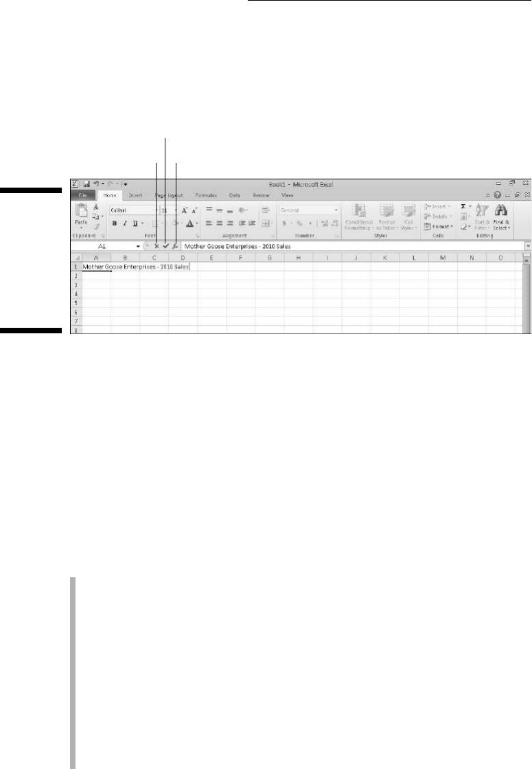
52
Part I: Getting In on the Ground Floor
As you continue to type, Excel displays your progress on the Formula bar
and in the active cell in the worksheet (see Figure 2-1). However, the inser-
tion point (the flashing vertical bar that acts as your cursor) displays only at
the end of the characters displayed in the cell.
Figure 2-1:
What
you type
appears
both in the
current cell
and on the
Formula bar.
Cancel
Enter
Insert function
After you finish typing your cell entry, you still have to get it into the cell so
that it stays put. When you do this, you also change the program from Enter
mode back to Ready mode so that you can move the cell pointer to another
cell and, perhaps, enter or edit the data there.
To complete your cell entry and, at the same time, get Excel out of Enter
mode and back into Ready mode, you can click the Enter button on the
Formula bar, press the Enter key, or press one of the arrow keys (↓, ↑, →, or
←) to move to another cell. You can also press the Tab key or Shift+Tab keys
to complete a cell entry.
Now, even though each of these alternatives gets your text into the cell, each
does something a little different afterward, so please take note:
✓ If you click the Enter button (the one with the check mark) on the
Formula bar, the text goes into the cell, and the cell pointer just stays in
the cell containing the brand-new entry.
✓ If you press the Enter key on your keyboard, the text goes into the cell,
and the cell pointer moves down to the cell below in the next row.
✓ If you press one of the arrow keys, the text goes into the cell, and the
cell pointer moves to the next cell in the direction of the arrow. Press
↓, and the cell pointer moves below in the next row just as it does when
you finish off a cell entry with the Enter key. Press → to move the cell
pointer right to the cell in the next column; press ← to move the cell
pointer left to the cell in the previous column; and press ↑ to move the
cell pointer up to the cell in the next row above.

53
Chapter 2: Creating a Spreadsheet from Scratch
✓ If you press Tab, the text goes into the cell, and the cell pointer moves
to the adjacent cell in the column on the immediate right (the same as
pressing the → key). If you press Shift+Tab, the cell pointer moves to the
adjacent cell in the column on the immediate left (the same as pressing
the ← key) after putting in the text.
No matter which of the methods you choose when putting an entry in its
place, as soon as you complete your entry in the current cell, Excel deacti-
vates the Formula bar by removing the Cancel and Enter buttons. Thereafter,
the data you entered continues to appear in the cell in the worksheet (with
certain exceptions that I discuss later in this chapter), and every time you
put the cell pointer into that cell, the data will reappear on the Formula bar
as well.
If, while still typing an entry or after finishing typing but prior to complet-
ing the entry, you realize that you’re just about to stick it in the wrong cell,
you can clear and deactivate the Formula bar by clicking the Cancel button
(the one with the X in it) or by pressing Esc. If, however, you don’t realize
that you had the wrong cell until after you enter your data there, you have to
either move the entry to the correct cell (something you find out how to do
in Chapter 4) or delete the entry (see Chapter 4) and then reenter the data in
the correct cell.
It Takes All Types
Unbeknownst to you while you go about happily entering data in your
spreadsheet, Excel constantly analyzes the stuff you type and classifies it into
one of three possible data types: a piece of text, a value, or a formula.
Getting the Enter key to put the cell
pointer where you want it
Excel automatically advances the cell pointer
to the next cell down in the column every time
you press Enter to complete the cell entry. If
you want to customize Excel so that pressing
Enter doesn’t move the cell pointer when the
program enters your data, or to have it move the
cell pointer to the next cell up, left, or right, open
the Advanced tab of the Excel Options dialog
box (Alt+FIA).
To prevent the cell pointer from moving at all,
select the After Pressing Enter, Move Selection
check box to remove its check mark. To have
the cell pointer move in another direction, click
the Direction pop-up list box right below and
then select the new direction you want to use
(Right, Up, or Left). When you finish changing
the settings, click OK or press Enter.

54
Part I: Getting In on the Ground Floor
If Excel finds that the entry is a formula, the program automatically calculates
the formula and displays the computed result in the worksheet cell (you con-
tinue to see the formula itself, however, on the Formula bar). If Excel is satis-
fied that the entry does not qualify as a formula (I give you the qualifications
for an honest-to-goodness formula a little later in this chapter), the program
then determines whether the entry should be classified as text or as a value.
Excel makes this distinction between text and values so that it knows how
to align the entry in the worksheet. It aligns text entries with the left edge of
the cell and values with the right edge. Because most formulas work prop-
erly only when they are fed values, by differentiating text from values, the
program knows which will and will not work in the formulas that you build.
Suffice to say that you can foul up your formulas but good if they refer to any
cells containing text where Excel expects values to be.
The telltale signs of text
A text entry is simply an entry that Excel can’t pigeonhole as either a for-
mula or value. This makes text the catchall category of Excel data types. As a
practical rule, most text entries (also known as labels) are a combination of
letters and punctuation or letters and numbers. Text is used mostly for titles,
headings, and notes in the worksheet.
You can tell right away whether Excel has accepted a cell entry as text
because text entries automatically align at the left edge of their cells. If the
text entry is wider than the cell can display, the data spills into the neigh-
boring cell or cells on the right, as long as those cells remain blank (see
Figure 2-2).
Figure 2-2:
Long text
entries spill
over into
neighboring
blank cells.
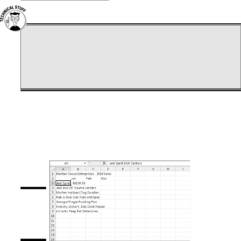
55
Chapter 2: Creating a Spreadsheet from Scratch
If, sometime later, you enter information in a cell that contains spillover text
from a cell to its left, Excel cuts off the spillover of the long text entry (see
Figure 2-3). Not to worry: Excel doesn’t actually lop these characters off the
cell entry — it simply shaves the display to make room for the new entry. To
redisplay the seemingly missing portion of the long text entry, you have to
widen the column that contains the cell where the text is entered. (To find
out how to do this, skip ahead to Chapter 3.)
Figure 2-3:
Entries in
cells to the
right cut off
the spillover
text in cells
on the left.
How Excel evaluates its values
Values are the building blocks of most of the formulas that you create in
Excel. As such, values come in two flavors: numbers that represent quantities
(14 stores or $140,000 dollars) and numbers that represent dates (July 30,
1995) or times (2 p.m.).
To Excel, text is nothing but a big zero
Use the AutoCalculate indicator to prove to
yourself that Excel gives all text entries the value
of 0 (zero). As an example, enter the number 10
in one cell and then some stupid piece of text,
such as Excel is like a box of chocolates, in
the cell directly below. Then drag up so that
both cells (the one with 10 and the one with
the text) are highlighted. Take a gander at the
AutoCalculate indicator on the Status bar, and
you see that it reads Average: 10, Count: 2, and
Sum: 10, proving that the text adds nothing to
the total value of these two cells.

56
Part I: Getting In on the Ground Floor
You can tell whether Excel has accepted your entry as a value because values
automatically align at the right edge of their cells. If the value that you enter
is wider than the column containing the cell can display, Excel automatically
converts the value to (of all things) scientific notation. To restore a value
that’s been converted into that weird scientific notation stuff to a regular
number, simply widen the column for that cell. (Read how in Chapter 3.)
Making sure that Excel’s got your number
When building a new worksheet, you’ll probably spend a lot of your time
entering numbers, representing all types of quantities from money that you
made (or lost) to the percentage of the office budget that went to coffee and
donuts. (You mean you don’t get donuts?)
To enter a numeric value that represents a positive quantity, like the amount
of money you made last year, just select a cell, type the numbers — for
example, 459600 — and complete the entry in the cell by clicking the Enter
button, pressing the Enter key, and so on. To enter a numeric value that rep-
resents a negative quantity, such as the amount of money the office spent on
coffee and donuts last year, begin the entry with the minus sign or hyphen
(–) before typing the numbers and then complete the entry. For example,
–175 (that’s not too much to spend on coffee and donuts when you just made
$459,600).
If you’re trained in accounting, you can enclose the negative number (that’s
expense to you) in parentheses. You’d enter it like this: (175). If you go to
all the trouble to use parentheses for your negatives (expenses), Excel goes
ahead and automatically converts the number so that it begins with a minus
sign; if you enter (175) in the Coffee and Donut expense cell, Excel spits back
–175. (Relax, you can find out how to get your beloved parentheses back for
the expenses in your spreadsheet in Chapter 3.)
With numeric values that represent dollar amounts, like the amount of money
you made last year, you can include dollar signs ($) and commas (,) just as
they appear in the printed or handwritten numbers you’re working from.
Just be aware that when you enter a number with commas, Excel assigns a
number format to the value that matches your use of commas. (For more
information on number formats and how they are used, see Chapter 3.)
Likewise, when you preface a financial figure with a dollar sign, Excel assigns
an appropriate dollar-number format to the value (one that automatically
inserts commas between the thousands).
When entering numeric values with decimal places, use the period as the
decimal point. When you enter decimal values, the program automatically
adds a zero before the decimal point (Excel inserts 0.34 in a cell when you
enter .34) and drops trailing zeros entered after the decimal point (Excel
inserts 12.5 in a cell when you enter 12.50).

57
Chapter 2: Creating a Spreadsheet from Scratch
If you don’t know the decimal equivalent for a value that contains a fraction,
you can just go ahead and enter the value with its fraction. For example, if
you don’t know that 2.1875 is the decimal equivalent for 2
3
⁄16, just type 2 3/16
(making sure to add a space between the 2 and 3) in the cell. After complet-
ing the entry, when you put the cell pointer in that cell, you see 2
3
⁄16 in the
cell of the worksheet, but 2.1875 appears on the Formula bar. As you see in
Chapter 3, it’s then a simple trick to format the display of 2
3
⁄16 in the cell so
that it matches the 2.1875 on the Formula bar.
If you need to enter simple fractions, such as ¾ or
5
⁄
8
, you must enter them as
a mixed number preceded by zero; for example, enter 0 3/4 or 0 5/8 (be sure
to include a space between the zero and the fraction). Otherwise, Excel thinks
that you’re entering the dates March 4 (3/4) and May 8 (5/8).
When entering in a cell a numeric value that represents a percentage (so
much out of a hundred), you have this choice:
✓ You can either divide the number by 100 and enter the decimal equiva-
lent (by moving the decimal point two places to the left like your teacher
taught you; for example, enter .12 for 12 percent).
✓ You can enter the number with the percent sign (for example, enter 12%).
Either way, Excel stores the decimal value in the cell (0.12 in this example).
If you use the percent sign, Excel assigns a percentage-number format to the
value in the worksheet so that it appears as 12%.
How to fix your decimal places (when you
don’t even know they’re broken)
If you find that you need to enter a whole slew of numbers that use the same
number of decimal places, you can turn on Excel’s Fixed Decimal setting and
have the program enter the decimals for you. This feature really comes in
handy when you have to enter hundreds of financial figures that all use two
decimal places (for example, for the number of cents).
To fix the number of decimal places in a numeric entry, follow these steps:
1. Choose File➪Options➪Advanced or press Alt+FIA.
The Advanced tab of the Excel Options dialog box opens.
2. Click the Automatically Insert a Decimal Point check box in the
Editing Options section to fill it with a check mark.
By default, Excel fixes the decimal place two places to the left of the last
number you type. To change the default Places setting, go to Step 3; oth-
erwise move to Step 4.

58
Part I: Getting In on the Ground Floor
3. (Optional) Type a new number in the Places text box or use the spin-
ner buttons to change the value.
For example, you could change the Places setting to 3 to enter numbers
with the following decimal placement: 00.000.
4. Click OK or press Enter.
Excel displays the Fixed Decimal status indicator on the Status bar to let
you know that the Fixed Decimal feature is now active.
After fixing the decimal place in numeric values, Excel automatically adds a
decimal point to any numeric value that you enter using the number of places
you selected; all you do is type the digits and complete the entry in the cell.
For example, to enter the numeric value 100.99 in a cell after fixing the deci-
mal point to two places, type the digits 10099 without adding any period
for a decimal point. When you complete the cell entry, Excel automatically
inserts a decimal point two places from the right in the number you typed,
leaving 100.99 in the cell.
When you’re ready to return to normal data entry for numerical values
(where you enter any decimal points yourself), open the Advanced tab of the
Excel Options dialog box (Alt+FIA), click the Automatically Insert a Decimal
Point check box again, this time to clear it, and then click OK or press Enter.
Excel removes the Fixed Decimal indicator from the Status bar.
Tapping on the old ten-key
You can make the Fixed Decimal feature work even better by selecting the
block of cells where you want to enter numbers (see “Entries all around the
block,” later in this chapter) and then pressing Num Lock so that you can
enter all the data for this cell selection from the numeric keypad (à la ten-key
adding machine).
Don’t get in a fix over your decimal places!
When the Fixed Decimal setting is on, Excel
adds a decimal point to all the numeric values
that you enter. However, if you want to enter
a number without a decimal point, or one with
a decimal point in a position different from
the one called for by this feature, you have to
remember to type the decimal point (period)
yourself. For example, to enter the number 1099
instead of 10.99 when the decimal point is fixed
at two places, type 1099 followed immediately
by a period (.) in the cell.
And, for heaven’s sake, please don’t forget
to turn off the Fixed Decimal feature before
you work on another worksheet or exit Excel.
Otherwise, when you intend to enter values,
such as 20, you’ll end up with 0.2 instead, and
you won’t have a clue what’s going on!
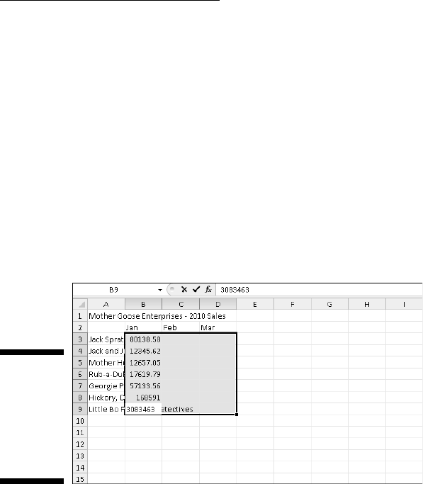
59
Chapter 2: Creating a Spreadsheet from Scratch
Using this approach, all you have to do to enter the range of values in each
cell is type the number’s digits and press Enter on the numeric keypad. Excel
inserts the decimal point in the proper place while it moves the cell pointer
down to the next cell. Even better, when you finish entering the last value in a
column, pressing Enter automatically moves the cell pointer to the cell at the
top of the next column in the selection.
Look at Figures 2-4 and 2-5 to see how you can make the ten-key method
work for you. In Figure 2-4, the Fixed Decimal feature is turned on (using the
default of two decimal places), and the block of cells from B3 through D9
are selected. You also see that six entries have already been made in cells
B3 through B8 and a seventh, 30834.63, is about to be completed in cell B9.
To make this entry when the Fixed Decimal feature is on, you simply type
3083463 from the numeric keypad.
Figure 2-4:
To enter
the value
30834.63 in
cell B9, type
3083463 and
press Enter.
In Figure 2-5, check out what happens when you press Enter (on either the
regular keyboard or the numeric keypad). Not only does Excel automati-
cally add the decimal point to the value in cell B9, but it also moves the cell
pointer up and over to cell C3 where you can continue entering the values for
this column.
Entering dates with no debate
At first look, it may strike you a bit odd to enter dates and times as values
in the cells of a worksheet rather than text. The reason for this is simple,
really: Dates and times entered as values can be used in formula calculations,
whereas dates and times entered as text cannot. For example, if you enter
two dates as values, you can then set up a formula that subtracts the more
recent date from the older date and returns the number of days between
them. This kind of thing just couldn’t happen if you were to enter the two
dates as text entries.

60
Part I: Getting In on the Ground Floor
Figure 2-5:
Press Enter
to complete
the 30834.63
entry in cell
B9. Excel
automati-
cally moves
the cell
pointer up
and over to
cell C3.
Excel determines whether the date or time that you type is a value or text
by the format that you follow. If you follow one of Excel’s built-in date and
time formats, the program recognizes the date or time as a value. If you don’t
follow one of the built-in formats, the program enters the date or time as a
text entry — it’s as simple as that.
Excel recognizes the following time formats:
3 AM or 3 PM
3 A or 3 P (upper- or lowercase a or p — Excel inserts 3:00 AM or
3:00 PM)
3:21 AM or 3:21 PM (upper- or lowercase am or pm)
3:21:04 AM or 3:21:04 PM (upper- or lowercase am or pm)
15:21
15:21:04
Excel isn’t fussy, so you can enter the AM or PM designation in the date in any
manner — uppercase letters, lowercase letters, or even a mix of the two.
Excel knows the following date formats. (Month abbreviations always use the
first three letters of the name of the month: Jan, Feb, Mar, and so forth.)
November 6, 2008 or November 6, 08 (appear in cell as 6-Nov-08)
11/6/08 or 11-6-08 (appear in cell as 11/6/2008)
6-Nov-08 or 6/Nov/08 or even 6Nov08 (all appear in cell as 6-Nov-08)
11/6 or 6-Nov or 6/Nov or 6Nov (all appear in cell as 6-Nov)
Nov-06 or Nov/06 or Nov06 (all appear in cell as 6-Nov)

61
Chapter 2: Creating a Spreadsheet from Scratch
Make it a date in the 21st Century
Contrary to what you might think, when entering dates in the 21st Century,
you need to enter only the last two digits of the year. For example, to enter
the date January 6, 2008, in a worksheet, I enter 1/6/08 in the target cell.
Likewise, to put the date February 15, 2010, in a worksheet, I enter 2/15/10 in
the target cell.
This system of having to put in only the last two digits of dates in the 21st
Century works only for dates in the first three decades of the new century
(2000 through 2029). To enter dates for the years 2030 on, you need to input
all four digits of the year.
This also means, however, that to put in dates in the first three decades
of the 20th Century (1900 through 1929), you must enter all four digits of
the year. For example, to put in the date July 21, 1925, you have to enter
7/21/1925 in the target cell. Otherwise, if you enter just the last two digits
(25) for the year part of the date, Excel enters a date for the year 2025 and
not 1925!
Excel 2010 always displays all four digits of the year in the cell and on the
Formula bar even when you only enter the last two. For example, if you enter
11/06/08 in a cell, Excel automatically displays 11/6/2008 in the worksheet
cell (and on the Formula bar when that cell is current).
Therefore, by looking at the Formula bar, you can always tell when you’ve
entered a 20th rather than a 21st Century date in a cell even if you can’t keep
straight the rules for when to enter just the last two digits rather than all
four. (Read Chapter 3 for information on how to format your date entries so
that only the last digits display in the worksheet.)
The dating game
Dates are stored as serial numbers that indi-
cate how many days have elapsed from a
particular starting date; times are stored as
decimal fractions indicating the elapsed part
of the 24-hour period. Excel supports two date
systems: the 1900 date system used by Excel in
Windows, where January 1, 1900 is the starting
date (serial number 1) and the 1904 system used
by Excel for the Macintosh, where January 2,
1904 is the starting date.
If you ever get a hold of a workbook created
with Excel for the Macintosh that contains
dates that seem all screwed up when you open
the file, you can rectify this problem by opening
the Advanced tab of the Excel Options dialog
box (File➪Options➪Advanced or Alt+FIA) and
then clicking the Use 1904 Date System check
box in the When Calculating This Workbook
section before you click OK.

62
Part I: Getting In on the Ground Floor
For information on how to perform simple arithmetic operations between the
dates and time you enter in a worksheet and have the results make sense, see
the information about dates in Chapter 3.
Fabricating those fabulous formulas!
As entries go in Excel, formulas are the real workhorses of the worksheet.
If you set up a formula properly, it computes the correct answer when you
enter the formula into a cell. From then on, the formula stays up to date,
recalculating the results whenever you change any of the values that the for-
mula uses.
You let Excel know that you’re about to enter a formula (rather than some
text or a value), in the current cell by starting the formula with the equal sign
(=). Most simple formulas follow the equal sign with a built-in function, such
as SUM or AVERAGE. (See the section “Inserting a function into a formula with
the Insert Function button,” later in this chapter, for more information on
using functions in formulas.) Other simple formulas use a series of values or
cell references that contain values separated by one or more of the following
mathematical operators:
+ (plus sign) for addition
– (minus sign or hyphen) for subtraction
* (asterisk) for multiplication
/ (slash) for division
^ (caret) for raising a number to an exponential power
For example, to create a formula in cell C2 that multiplies a value entered in
cell A2 by a value in cell B2, enter the following formula in cell C2: =A2*B2.
To enter this formula in cell C2, follow these steps:
1. Select cell C2.
2. Type the entire formula =A2*B2 in the cell.
3. Press Enter.
Or
1. Select cell C2.
2. Type = (equal sign).
3. Select cell A2 in the worksheet by using the mouse or the keyboard.
This action places the cell reference A2 in the formula in the cell (as
shown in Figure 2-6).
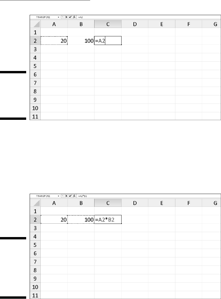
63
Chapter 2: Creating a Spreadsheet from Scratch
Figure 2-6:
To start the
formula,
type = and
then select
cell A2.
4. Type * (Shift+8 on the top row of the keyboard).
The asterisk is used for multiplication rather than the × symbol you
used in school.
5. Select cell B2 in the worksheet by using the mouse or the keyboard.
This action places the cell reference B2 in the formula (as shown in
Figure 2-7).
Figure 2-7:
To complete
the second
part of the
formula,
type * and
select
cell B2.
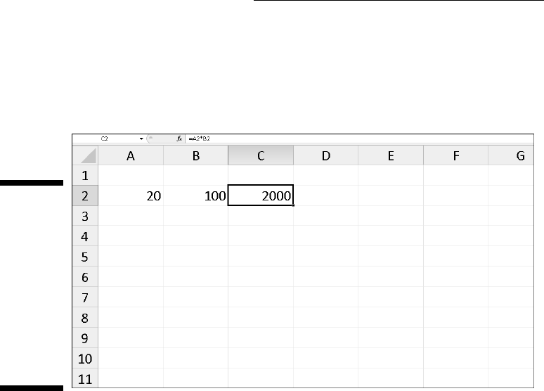
64
Part I: Getting In on the Ground Floor
6. Click the Enter button to complete the formula entry while keeping
the cell pointer in cell C2.
Excel displays the calculated answer in cell C2 and the formula =A2*B2
in the Formula bar (as shown in Figure 2-8).
Figure 2-8:
Click the
Enter but-
ton, and
Excel dis-
plays the
answer in
cell C2 while
the formula
appears in
the Formula
bar above.
When you finish entering the formula =A2*B2 in cell C2 of the worksheet,
Excel displays the calculated result, depending on the values currently
entered in cells A2 and B2. The major strength of the electronic spreadsheet
is the capability of formulas to change their calculated results automatically
to match changes in the cells referenced by the formulas.
Now comes the fun part: After creating a formula like the preceding one
that refers to the values in certain cells (rather than containing those values
itself), you can change the values in those cells, and Excel automatically
recalculates the formula, using these new values and displaying the updated
answer in the worksheet! Using the example shown in Figure 2-8, suppose
that you change the value in cell B2 from 100 to 50. The moment that you
complete this change in cell B2, Excel recalculates the formula and displays
the new answer, 1000, in cell C2.
If you want it, just point it out
The method of selecting the cells you use in a formula, rather than typing
their cell references, is pointing. Pointing is quicker than typing and reduces
the risk that you might mistype a cell reference. When you type a cell refer-
ence, you can easily type the wrong column letter or row number and not
realize your mistake by looking at the calculated result returned in the cell.

65
Chapter 2: Creating a Spreadsheet from Scratch
If you select the cell that you want to use in a formula either by clicking it or
moving the cell pointer to it, you have less chance of entering the wrong cell
reference.
Altering the natural order of operations
Many formulas that you create perform more than one mathematical opera-
tion. Excel performs each operation, moving from left to right, according to
a strict pecking order (the natural order of arithmetic operations). In this
order, multiplication and division pull more weight than addition and sub-
traction and, therefore, perform first, even if these operations don’t come
first in the formula (when reading from left to right).
Consider the series of operations in the following formula:
=A2+B2*C2
If cell A2 contains the number 5, B2 contains the number 10, and C2 contains
the number 2, Excel evaluates the following formula:
=5+10*2
In this formula, Excel multiplies 10 times 2 to equal 20 and then adds this
result to 5 to produce the result 25.
If you want Excel to perform the addition between the values in cells A2 and
B2 before the program multiplies the result by the value in cell C2, enclose
the addition operation in parentheses as follows:
=(A2+B2)*C2
The parentheses around the addition tell Excel that you want this operation
performed before the multiplication. If cell A2 contains the number 5, B2 con-
tains the number 10, and C2 contains the number 2, Excel adds 5 and 10 to
equal 15 and then multiplies this result by 2 to produce the result 30.
In fancier formulas, you may need to add more than one set of parentheses,
one within another (like the wooden Russian dolls that nest within each
other) to indicate the order in which you want the calculations to take place.
When nesting parentheses, Excel first performs the calculation contained in
the most inside pair of parentheses and then uses that result in further cal-
culations as the program works its way outward. For example, consider the
following formula:
=(A4+(B4–C4))*D4

66
Part I: Getting In on the Ground Floor
Excel first subtracts the value in cell C4 from the value in cell B4, adds the
difference to the value in cell A4, and then finally multiplies that sum by the
value in D4.
Without the additions of the two sets of nested parentheses, left to its own
devices, Excel would first multiply the value in cell C4 by that in D4, add the
value in A4 to that in B4, and then perform the subtraction.
Don’t worry too much when nesting parentheses in a formula if you don’t
pair them properly so that you have a right parenthesis for every left paren-
thesis in the formula. If you do not include a right parenthesis for every left
one, Excel displays an alert dialog box that suggests the correction needed to
balance the pairs. If you agree with the program’s suggested correction, you
simply click the Yes button. However, be sure that you only use parentheses:
( ). Excel balks at the use of brackets — [ ] — or braces — { } — in a formula
by giving you an Error alert box.
Formula flub-ups
Under certain circumstances, even the best formulas can appear to have
freaked out after you get them in your worksheet. You can tell right away that
a formula’s gone haywire because instead of the nice calculated value you
expected to see in the cell, you get a strange, incomprehensible message in all
uppercase letters beginning with the number sign (#) and ending with an excla-
mation point (!) or, in one case, a question mark (?). This weirdness, in the
parlance of spreadsheets, is as an error value. Its purpose is to let you know
that some element — either in the formula itself or in a cell referred to by the
formula — is preventing Excel from returning the anticipated calculated value.
When one of your formulas returns one of these error values, an alert indica-
tor (in the form of an exclamation point in a diamond) appears to the left of
the cell when it contains the cell pointer, and the upper-left corner of the cell
contains a tiny green triangle. When you position the mouse pointer on this
alert indicator, Excel displays a brief description of the formula error and adds
a drop-down button to the immediate right of its box. When you click this
button, a pop-up menu appears with a number of related options. To access
online help on this formula error, including suggestions on how to get rid of
the error, click the Help on This Error item on this pop-up menu.
The worst thing about error values is that they can contaminate other formu-
las in the worksheet. If a formula returns an error value to a cell and a second
formula in another cell refers to the value calculated by the first formula, the
second formula returns the same error value, and so on down the line.
After an error value shows up in a cell, you have to discover what caused
the error and edit the formula in the worksheet. In Table 2-1, I list some error
values that you might run into in a worksheet and then explain the most
common causes.

67
Chapter 2: Creating a Spreadsheet from Scratch
Table 2-1 Error Values That You May Encounter
from Faulty Formulas
What Shows Up
in the Cell
What’s Going On Here?
#DIV/0! Appears when the formula calls for division by a cell that
either contains the value 0 or, as is more often the case, is
empty. Division by zero is a no-no in mathematics.
#NAME? Appears when the formula refers to a range name (see
Chapter 6 for info on naming ranges) that doesn’t exist in the
worksheet. This error value appears when you type the wrong
range name or fail to enclose in quotation marks some text
used in the formula, causing Excel to think that the text refers
to a range name.
#NULL! Appears most often when you insert a space (where you
should have used a comma) to separate cell references used
as arguments for functions.
#NUM! Appears when Excel encounters a problem with a number in
the formula, such as the wrong type of argument in an Excel
function or a calculation that produces a number too large or
too small to be represented in the worksheet.
#REF! Appears when Excel encounters an invalid cell reference,
such as when you delete a cell referred to in a formula or
paste cells over the cells referred to in a formula.
#VALUE! Appears when you use the wrong type of argument or opera-
tor in a function, or when you call for a mathematical opera-
tion that refers to cells that contain text entries.
Fixing Those Data Entry Flub-Ups
We all wish we were perfect, but alas, because so few of us are, we are best
off preparing for those inevitable times when we mess up. When entering
vast quantities of data, it’s easy for those nasty little typos to creep into your
work. In your pursuit of the perfect spreadsheet, here are things you can do.
First, get Excel to correct certain data entry typos automatically when they
happen with its AutoCorrect feature. Second, manually correct any disgust-
ing little errors that get through, either while you’re still in the process of
making the entry in the cell or after the entry has gone in.

68
Part I: Getting In on the Ground Floor
You really AutoCorrect that for me
The AutoCorrect feature is a godsend for those of us who tend to make the
same stupid typos over and over. With AutoCorrect, you can alert Excel 2010
to your own particular typing gaffes and tell the program how it should auto-
matically fix them for you.
When you first install Excel, the AutoCorrect feature already knows to auto-
matically correct two initial capital letters in an entry (by lowercasing the
second capital letter), to capitalize the name of the days of the week, and to
replace a set number of text entries and typos with particular substitute text.
You can add to the list of text replacements at any time when using Excel.
These text replacements can be of two types: typos that you routinely make
along with the correct spelling, and abbreviations or acronyms that you type
all the time along with their full forms.
To add to the replacements:
1. Choose File➪Options➪Proofing or press Alt+FIP and then click the
AutoCorrect Options button or press Alt+A.
Excel opens the AutoCorrect dialog box shown in Figure 2-9.
2. On the AutoCorrect tab in this dialog box, enter the typo or abbrevia-
tion in the Replace text box.
3. Enter the correction or full form in the With text box.
4. Click the Add button or press Enter to add the new typo or abbrevia-
tion to the AutoCorrect list.
5. Click the OK button to close the AutoCorrect dialog box.
Figure 2-9:
Use the
Replace and
With options
in the
AutoCorrect
dialog box
to add all
typos and
abbre-
viations you
want Excel
to automati-
cally correct
or fill out.

69
Chapter 2: Creating a Spreadsheet from Scratch
Cell editing etiquette
Despite the help of AutoCorrect, some mistakes are bound to get you. How
you correct them really depends upon whether you notice before or after
completing the cell entry.
✓ If you catch the mistake before you complete an entry, you can delete
it by pressing your Backspace key until you remove all the incorrect
characters from the cell. Then you can retype the rest of the entry or the
formula before you complete the entry in the cell.
✓ If you don’t discover the mistake until after you’ve completed the cell
entry, you have a choice of replacing the whole thing or editing just the
mistakes.
✓ When dealing with short entries, you’ll probably want to take the
replacement route. To replace a cell entry, position the cell pointer in
that cell, type your replacement entry, and then click the Enter button
or press one of the arrow keys.
✓ When the error in an entry is relatively easy to fix and the entry is on the
long side, you’ll probably want to edit the cell entry rather than replace
it. To edit the entry in the cell, simply double-click the cell or select the
cell and then press F2.
✓ Doing either one reactivates the Formula bar by displaying the Enter
and Cancel buttons once again and placing the insertion point in the cell
entry in the worksheet. (If you double-click, the insertion point positions
itself wherever you click; press F2, and the insertion point positions
itself after the last character in the entry.)
✓ Notice also that the mode indicator changes to Edit. While in this mode,
you can use the mouse or the arrow keys to position the insertion point
at the place in the cell entry that needs fixing.
In Table 2-2, I list the keystrokes that you can use to reposition the inser-
tion point in the cell entry and delete unwanted characters. If you want to
insert new characters at the insertion point, simply start typing. If you want
to delete existing characters at the insertion point while you type new ones,
press the Insert key on your keyboard to switch from the normal insert mode
to overtype mode. To return to normal insert mode, press Insert a second
time. When you finish making corrections to the cell entry, you must com-
plete the edits by pressing Enter before Excel updates the contents of the
cell.
While Excel is in Edit mode, you must reenter the edited cell contents by
either clicking the Enter button or pressing Enter. You can use the arrow keys
as a way to complete an entry only when the program is in Enter mode. When
the program is in Edit mode, the arrow keys move the insertion point only
through the entry that you’re editing, not to a new cell.

70
Part I: Getting In on the Ground Floor
Table 2-2 Keystrokes for Fixing Those Cell Entry Flub-Ups
Keystroke What the Keystroke Does
Delete Deletes the character to the right of the insertion point
Backspace Deletes the character to the left of the insertion point
→
Positions the insertion point one character to the right
←
Positions the insertion point one character to the left
↑
Positions the insertion point, when it is at the end of the
cell entry, to its preceding position to the left
End or ↓
Moves the insertion point after the last character in the
cell entry
Home Moves the insertion point in front of the first character of
the cell entry
Ctrl+→
Positions the insertion point in front of the next word in the
cell entry
Ctrl+←
Positions the insertion point in front of the preceding word
in the cell entry
Insert Switches between insert and overtype mode
A tale of two edits: Cell versus Formula bar editing
Excel gives you a choice between editing
a cell’s contents either in the cell or on the
Formula bar. Whereas most of the time, editing
right in the cell is just fine, when dealing with
really long entries (like humongous formulas
that go on forever or text entries that take up
paragraphs), you may prefer to do your editing
on the Formula bar. This is because Excel 2010
automatically adds up and down scroll arrow
buttons to the end of the Formula bar when a
cell entry is too long to display completely on a
single row. These scroll arrow buttons enable
you to display each line of the cell’s long entry
without expanding the Formula bar (as in earlier
versions of Excel) and thereby obscuring the
top part of the Worksheet area.
To edit the contents in the Formula bar rather
than in the cell itself, click the appropriate
scroll arrow button to display the line with the
contents that needs editing and then click the
I-beam mouse pointer at the place in the text
or numbers that requires modification to set the
insertion cursor.

71
Chapter 2: Creating a Spreadsheet from Scratch
Taking the Drudgery out of Data Entry
Before leaving the topic of data entry, I feel duty-bound to cover some of the
shortcuts that really help to cut down on the drudgery of this task. These
data-entry tips include AutoComplete and AutoFill features as well as doing
data entry in a preselected block of cells and making the same entry in a
bunch of cells all at the same time.
I’m just not complete without you
The AutoComplete feature in Excel 2010 is not something you can do any-
thing about, just something to be aware of while you enter your data. In an
attempt to cut down on your typing load, our friendly software engineers at
Microsoft came up with the AutoComplete feature.
AutoComplete is like a moronic mind reader who anticipates what you might
want to enter next based on what you just entered. This feature comes into
play only when you’re entering a column of text entries. (It does not come
into play when entering values or formulas or when entering a row of text
entries.) When entering a column of text entries, AutoComplete looks at the
kinds of entries that you make in that column and automatically duplicates
them in subsequent rows whenever you start a new entry that begins with
the same letter as an existing entry.
For example, suppose that I enter Jack Sprat Diet Centers (one of the compa-
nies owned and operated by Mother Goose Enterprises) in cell A2 and then
move the cell pointer down to cell A3 in the row below and press J (lower-
case or uppercase, it doesn’t matter). AutoComplete immediately inserts the
remainder of the familiar entry — ack Sprat Diet Centers — in this cell after
the J, as shown in Figure 2-10.
Now this is great if I happen to need Jack Sprat Diet Centers as the row
heading in both cells A2 and A3. Anticipating that I might be typing a differ-
ent entry that just happens to start with the same letter as the one above,
AutoComplete automatically selects everything after the first letter in the
duplicated entry it inserted (from ack on, in this example). This enables me
to replace the duplicate text supplied by AutoComplete just by continuing
to type. For example, after capturing the Excel screen that you see in Figure
2-10, I entered Jack and Jill Trauma Centers — another of Mother’s compa-
nies — in cell A3.
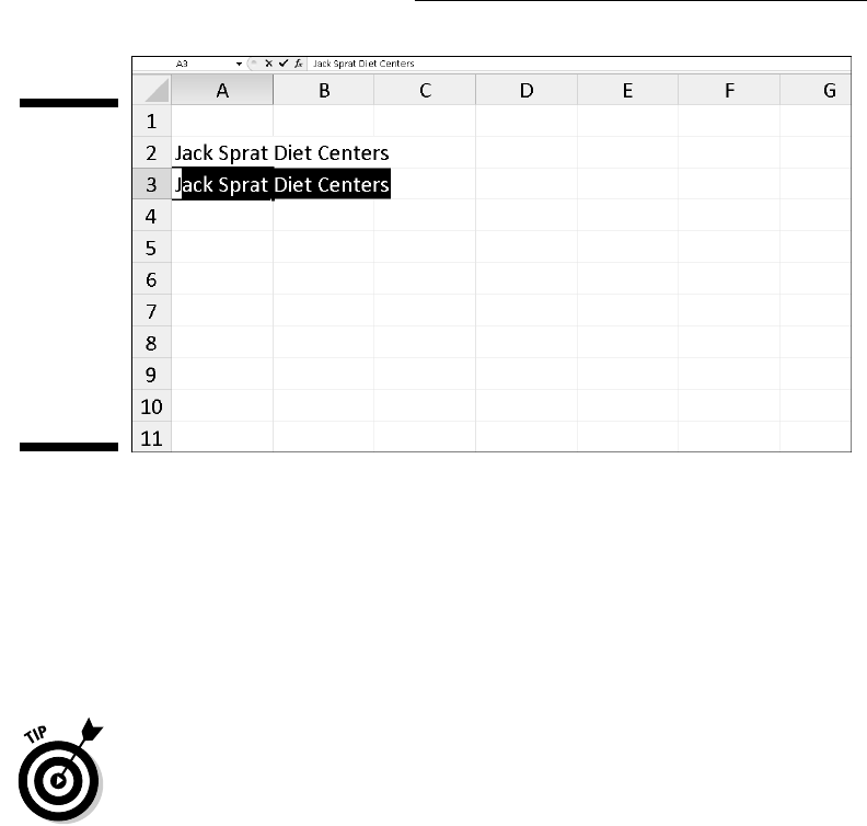
72
Part I: Getting In on the Ground Floor
Figure 2-10:
Auto
Complete
duplicates
a previous
entry if you
start a new
entry in
the same
column that
begins with
the same
letter.
If you override a duplicate supplied by AutoComplete in a column by typing
one of your own (as in my example with changing Jack Sprat Diet Centers to
Jack and Jill Trauma Centers in cell A3), you effectively shut down its abil-
ity to supply any more duplicates for that particular letter. For instance, in
my example, after changing Jack Sprat Diet Centers to Jack and Jill Trauma
Centers in cell A3, AutoComplete doesn’t do anything if I then type J in
cell A4. In other words, you’re on your own if you don’t continue to accept
AutoComplete’s typing suggestions.
If you find that the AutoComplete feature is really making it hard for you
to enter a series of cell entries that all start with the same letter but are
otherwise not alike, you can turn off the AutoComplete feature. Click
File➪Options➪Advanced or press Alt+FIA to select the Advanced tab of the
Excel Options dialog box. Then, select the Enable AutoComplete for Cell
Values check box in the Editing Options section to remove its check mark
before clicking OK.
Fill ’er up with AutoFill
Many of the worksheets that you create with Excel require the entry of
a series of sequential dates or numbers. For example, a worksheet may
require you to title the columns with the 12 months, from January through
December, or to number the rows from 1 to 100.
Excel’s AutoFill feature makes short work of this kind of repetitive task. All
you have to enter is the starting value for the series. In most cases, AutoFill
is smart enough to figure out how to fill out the series for you when you drag
the fill handle to the right (to take the series across columns to the right) or
down (to extend the series to the rows below).

73
Chapter 2: Creating a Spreadsheet from Scratch
The AutoFill handle looks like this — + — and appears only when you posi-
tion the mouse pointer on the lower-right corner of the active cell (or the last
cell, when you’ve selected a block of cells). If you drag a cell selection with
the white cross mouse pointer rather than the AutoFill handle, Excel simply
extends the cell selection to those cells you drag through (see Chapter 3).
If you drag a cell selection with the arrowhead pointer, Excel moves the cell
selection (see Chapter 4).
When creating a series with the fill handle, you can drag in only one direction
at a time. For example, you can fill the series or copy the entry to the range
to the left or right of the cell that contains the initial values, or you can fill
the series or copy to the range above or below the cell containing the initial
values. You can’t, however, fill or copy the series to two directions at the same
time (such as down and to the right by dragging the fill handle diagonally).
While you drag the mouse, the program keeps you informed of whatever
entry will be entered into the last cell selected in the range by displaying that
entry next to the mouse pointer (a kind of AutoFill tips, if you will). When
you release the mouse button after extending the range with the fill handle,
Excel either creates a series in all of the cells that you select or copies the
entire range with the initial value. To the right of the last entry in the filled
or copied series, Excel also displays a drop-down button that contains a
shortcut menu of options. You can use this shortcut menu to override Excel’s
default filling or copying. For example, when you use the fill handle, Excel
copies an initial value into a range of cells. But, if you want a sequential
series, you could do this by selecting the Fill Series command on the AutoFill
Options shortcut menu.
In Figures 2-11 and 2-12, I illustrate how to use AutoFill to enter a row of
months, starting with January in cell B2 and ending with June in cell G2. To
do this, you simply enter January in cell B2 and then position the mouse
pointer on the fill handle in the lower-right corner of this cell before you drag
through to cell G2 on the right (as shown in Figure 2-11). When you release
the mouse button, Excel fills in the names of the rest of the months (February
through June) in the selected cells (as shown in Figure 2-12). Excel keeps the
cells with the series of months selected, giving you another chance to modify
the series. (If you went too far, you can drag the fill handle to the left to cut
back on the list of months; if you didn’t go far enough, you can drag it to the
right to extend the list of months further.)
Also, you can use the options on the AutoFill Options drop-down menu
(opened by clicking the drop-down button that appears on the fill handle to
the right of June) to override the series created by default. To have Excel
copy January into each of the selected cells, choose Copy Cells on this menu.
To have the program fill the selected cells with the formatting used in cell B2
(in this case, the cell has had bold applied to it — see Chapter 3 for details on
formatting cells), you select Fill Formatting Only on this menu. To have Excel
fill in the series of months in the selected cells without copying the format-
ting used in cell B2, you select the Fill without Formatting command from this
shortcut menu.
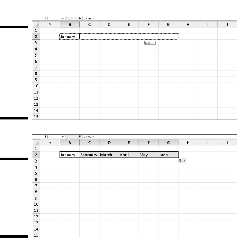
74
Part I: Getting In on the Ground Floor
Figure 2-11:
To enter a
series of
months,
enter the
first month
and then
drag the Fill
handle in a
direction to
add sequen-
tial months.
Figure 2-12:
Release
the mouse
button, and
Excel fills
the cell
selection
with the
missing
months.
See Table 2-3 in the following section to see some of the different initial
values that AutoFill can use and the types of series that Excel can create from
them.
Working with a spaced series
AutoFill uses the initial value that you select (date, time, day, year, and so
on) to design the series. All the sample series I show in Table 2-3 change by
a factor of one (one day, one month, or one number). You can tell AutoFill to
create a series that changes by some other value: Enter two sample values
in neighboring cells that describe the amount of change you want between
each value in the series. Make these two values the initial selection that you
extend with the fill handle.

75
Chapter 2: Creating a Spreadsheet from Scratch
For example, to start a series with Saturday and enter every other day across
a row, enter Saturday in the first cell and Monday in the cell next door. After
selecting both cells, drag the fill handle across the cells to the right as far
as you need to fill out a series based on these two initial values. When you
release the mouse button, Excel follows the example set in the first two cells
by entering every other day (Wednesday to the right of Monday, Friday to the
right of Wednesday, and so on).
Table 2-3 Samples of Series You Can Create with AutoFill
Value Entered
in First Cell
Extended Series Created by AutoFill in the Next Three Cells
June July, August, September
Jun Jul, Aug, Sep
Tuesday Wednesday, Thursday, Friday
Tue Wed, Thu, Fri
4/1/99 4/2/99, 4/3/99, 4/4/99
Jan-00 Feb-00, Mar-00, Apr-00
15-Feb 16-Feb, 17-Feb, 18-Feb
10:00 PM 11:00 PM, 12:00 AM, 1:00 AM
8:01 9:01, 10:01, 11:01
Quarter 1 Quarter 2, Quarter 3, Quarter 4
Qtr2 Qtr3, Qtr4, Qtr1
Q3 Q4, Q1, Q2
Product 1 Product 2, Product 3, Product 4
Copying with AutoFill
You can use AutoFill to copy a text entry throughout a cell range (rather
than fill in a series of related entries). To copy a text entry to a cell range,
hold down the Ctrl key while you click and drag the Fill handle. When you
hold down the Ctrl key while you click the fill handle, a plus sign appears to
the right of the Fill handle — your sign that AutoFill will copy the entry in the
active cell instead of creating a series using it. You can also tell because the
entry that appears as the AutoFill tip next to the mouse pointer while you
drag contains the same text as the original cell. If you decide after copying an
initial label or value to a range that you should have used it to fill in a series,
click the drop-down button that appears on the fill handle at the cell with
the last copied entry and then select the Fill Series command on the AutoFill
Options shortcut menu that appears.

76
Part I: Getting In on the Ground Floor
Although holding down Ctrl while you drag the fill handle copies a text entry,
just the opposite is true when it comes to values! Suppose that you enter the
number 17 in a cell and then drag the fill handle across the row — Excel just
copies the number 17 in all the cells that you select. If, however, you hold
down Ctrl while you drag the fill handle, Excel then fills out the series (17, 18,
19, and so on). If you forget and create a series of numbers when you only
need the value copied, rectify this situation by selecting the Copy Cells com-
mand on the AutoFill Options shortcut menu.
Creating custom lists for AutoFill
In addition to varying the increment in a series created with AutoFill, you
can also create your own custom series. For example, say your company has
offices in the following locations and you get tired of typing the sequence in
each new spreadsheet that requires them:
✓ New York
✓ Chicago
✓ Atlanta
✓ Seattle
✓ San Francisco
✓ San Diego
After creating a custom list with these locations, you can enter the entire
sequence of cities simply by entering New York in the first cell and then drag-
ging the Fill handle to the blank cells where the rest of the companies should
appear.
To create this kind of custom series, follow these steps:
1. Choose File➪Options➪Advanced or press Alt+FIA and then click the
Edit Custom Lists button in the General section to open the Options
dialog box (as shown in Figure 2-13).
If you’ve already gone to the time and trouble of typing the custom list
in a range of cells, go to Step 2. If you haven’t yet typed the series in an
open worksheet, go to Step 5.
2. Click inside the Import List from Cells text box and then click the
Collapse Dialog Box button (the one with the picture of the tiny grid
to the right of the Import List from Cells text box) so that you can
see your list and drag through the range of cells to select them (see
Chapter 3 for details).
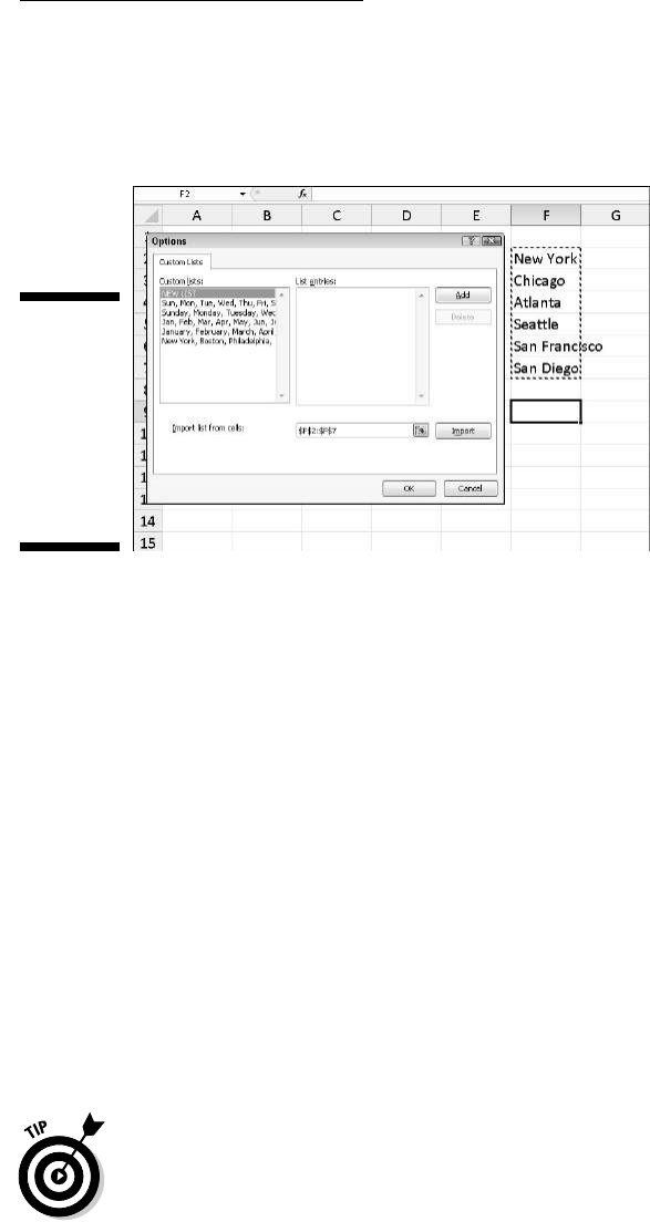
77
Chapter 2: Creating a Spreadsheet from Scratch
3. After selecting the cells in the worksheet, click the Expand Dialog Box
button.
This button automatically replaces the Collapse Dialog Box button.
Figure 2-13:
Creating
a custom
company
location
list from a
range of
existing cell
entries.
4. Click the Import button to copy this list into the List Entries list box.
Skip to Step 7.
5. Click inside the List Entries list box and then type each entry (in the
desired order), being sure to press Enter after typing each one.
When all the entries in the custom list appear in the List Entries list box
in the order you want them, proceed to Step 6.
6. Click the Add button to add the list of entries to the Custom Lists
list box.
Finish creating all the custom lists you need, using the preceding steps.
When you’re done, move to Step 7.
7. Click OK twice, the first time to close the Options dialog box and the
second to close the Excel Options dialog box and return to the current
worksheet in the active workbook.
After adding a custom list to Excel, from then on you need only enter the first
entry in a cell and then use the fill handle to extend it to the cells below or to
the right.
If you don’t even want to bother with typing the first entry, use the
AutoCorrect feature — refer to the section “You really AutoCorrect that for
me,” earlier in this chapter — to create an entry that will fill in as soon as you
type your favorite acronym for it (such as ny for New York).
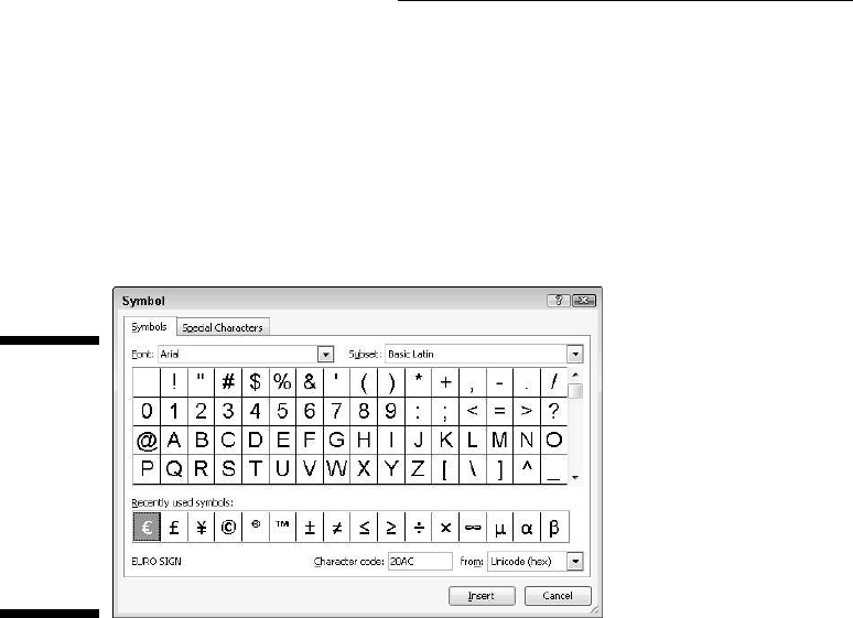
78
Part I: Getting In on the Ground Floor
Inserting special symbols
Excel makes it easy to enter special symbols, such as foreign currency indica-
tors, and special characters, such as the trademark and copyright symbols,
into your cell entries. To add a special symbol or character to a cell entry
you’re making or editing, click Insert➪Symbol on the Ribbon or press Alt+NU
to open the Symbol dialog box (similar to the one shown in Figure 2-14).
Figure 2-14:
Use the
Symbol
dialog box
to insert
special
symbols and
characters
into your
cell entries.
The Symbol dialog box contains two tabs: Symbols and Special Characters.
To insert a mathematical or foreign currency symbol on the Symbols tab,
click its symbol in the list box and then click the Insert button. (You can also
do this by double-clicking the symbol.) To insert characters, such as foreign
language or accented characters from other character sets, click the Subset
drop-down button, click the name of the set in the drop-down list, and then
click the desired characters in the list box. You can also insert commonly
used currency and mathematical symbols, such as the pound or plus-or-
minus symbol, by clicking them in the Recently Used Symbols section at the
bottom of this tab.
To insert special characters, such as the registered trademark, paragraph
symbol, and ellipsis, click the Special Characters tab of the Symbol dialog
box, locate the symbol in the scrolling list, click it, and then click the Insert
button. (You can insert one of these special characters by double-clicking it
also.)
When you finish inserting special symbols and characters, close the Symbol
dialog box by clicking its Close button in its upper-right corner.

79
Chapter 2: Creating a Spreadsheet from Scratch
Entries all around the block
When you want to enter a table of information in a new worksheet, you can
simplify the job of entering the data if you select all the empty cells in which
you want to make entries before you begin entering any information. Just
position the cell pointer in the first cell of what is to become the data table
and then select all the cells in the subsequent columns and rows. (For infor-
mation on the ways to select a range of cells, see Chapter 3.) After you select
the block of cells, you can begin entering the first entry.
When you select a block of cells (also known as a range) before you enter
information, Excel restricts data entry to that range as follows:
✓ The program automatically advances the cell pointer to the next cell in
the range when you click the Enter button or press Enter to complete
each cell entry.
✓ In a cell range that contains several different rows and columns, Excel
advances the cell pointer down each row of the column while you make
your entries. When the cell pointer reaches the cell in the last row of the
column, the cell pointer advances to the first selected row in the next
column to the right. If the cell range uses only one row, Excel advances
the cell pointer from left to right across the row.
✓ When you finish entering information in the last cell in the selected range,
Excel positions the cell pointer in the first cell of the now-completed data
table. To deselect the cell range, click the mouse pointer on one of the
cells in the worksheet (inside or outside the selected range — it doesn’t
matter) or press one of the arrow keys.
Be sure that you don’t press one of the arrow keys to complete a cell entry
within a preselected cell range instead of clicking the Enter button or pressing
Enter. Pressing an arrow key deselects the range of cells when Excel moves
the cell pointer. To move the cell pointer around a cell range without deselect-
ing the range, try these methods:
✓ Press Enter to advance to the next cell down each row and then across
each column in the range. Press Shift+Enter to move up to the previous
cell.
✓ Press Tab to advance to the next cell in the column on the right and
then down each row of the range. Press Shift+Tab to move left to the
previous cell.
✓ Press Ctrl+. (period) to move from one corner of the range to another.

80
Part I: Getting In on the Ground Floor
Data entry express
You can save a lot of time and energy when you want the same entry (text,
value, or formula) to appear in many cells of the worksheet; you can enter
the information in all the cells in one operation. You first select the cell
ranges to hold the information. (Excel lets you select more than one cell
range for this kind of thing — see Chapter 3 for details.) Then you construct
the entry on the formula bar and press Ctrl+Enter to put the entry into all the
selected ranges.
The key to making this operation a success is to hold the Ctrl key while you
press Enter so that Excel inserts the entry on the formula bar into all the
selected cells. If you forget to hold Ctrl and you just press Enter, Excel places
the entry in the first cell only of the selected cell range.
You can also speed up data entry in a list that includes formulas by making
sure that the Extend Data Range Formats and Formulas check box is selected
in the Editing Options section of the Advanced tab in the Excel Options dialog
box. (Choose File➪Options➪Advanced or press Alt+FIA.) When this check
box is selected, Excel automatically formats new data that you type in the
last row of a list to match that of like data in earlier rows and copies down
formulas that appear in the preceding rows. Note, however, that for this new
feature to kick in, you must manually enter the formulas and format the data
entries in at least three rows preceding the new row.
How to Make Your Formulas
Function Even Better
Earlier in this chapter, I show you how to create formulas that perform a
series of simple mathematical operations, such as addition, subtraction, mul-
tiplication, and division. (See the section “Fabricating those fabulous formu-
las!”) Instead of creating complex formulas from scratch out of an intricate
combination of these operations, you can find an Excel function to get the job
done.
A function is a predefined formula that performs a particular type of com-
putation. All you have to do to use a function is supply the values that the
function uses when performing its calculations. (In the parlance of the
Spreadsheet Guru, such values are the arguments of the function.) As with
simple formulas, you can enter the arguments for most functions either as a
numerical value (for example, 22 or –4.56) or, as is more common, as a cell
reference (B10) or as a cell range (C3:F3).

81
Chapter 2: Creating a Spreadsheet from Scratch
Just as with a formula you build yourself, each function you use must start
with an equal sign (=) so that Excel knows to enter the function as a formula
rather than as text. Following the equal sign, you enter the name of the func-
tion (in uppercase or lowercase — it doesn’t matter, as long as you spell the
name correctly). Following the name of the function, you enter the arguments
required to perform the calculations. All function arguments are enclosed in
a pair of parentheses.
If you type the function directly in a cell, remember not to insert spaces
between the equal sign, function name, and the arguments enclosed in paren-
theses. Some functions use more than one value when performing their des-
ignated calculations. When this is the case, you separate each function with a
comma (not a space).
After you type the equal sign and begin typing the first few letters of the
name of the function you want to use, a drop-down list showing all the func-
tions that begin with the letters you’ve typed appears immediately beneath
the cell. When you see the name of the function you want to use on this list,
double-click it and Excel will finish entering the function name in the cell and
on the Formula bar as well as add the left parenthesis that marks the begin-
ning of the arguments for the function.
Excel then displays all the arguments that the function takes beneath the cell
and you can indicate any cell or cell range that you want to use as the first
argument by either pointing to it or typing its cell or range references. When
the function uses more than one argument, you can point to the cells or cell
ranges or enter the addresses for the second argument right after you enter a
comma (,) to complete the first argument.
After you finish entering the last argument, you need to close off the func-
tion by typing a right parenthesis to mark the end of the argument list. The
display of the function name along with its arguments that appeared beneath
the cell when you first selected the function from the drop-down list then dis-
appears. Click the Enter button or press Enter (or the appropriate arrow key)
to then insert the function into the cell and have Excel calculate the answer.
Inserting a function into a formula with
the Insert Function button
Although you can enter a function by typing it directly in a cell, Excel pro-
vides an Insert Function button on the Formula bar you can use to select
any of Excel’s functions. When you click this button, Excel opens the Insert
Function dialog box (shown in Figure 2-15) where you can select the function
you want to use. After you select your function, Excel opens the Function
Arguments dialog box. In this dialog box, you can specify the function argu-
ments. The real boon comes when you’re fooling with an unfamiliar function
or one that’s kind of complex (some of these puppies can be hairy). You
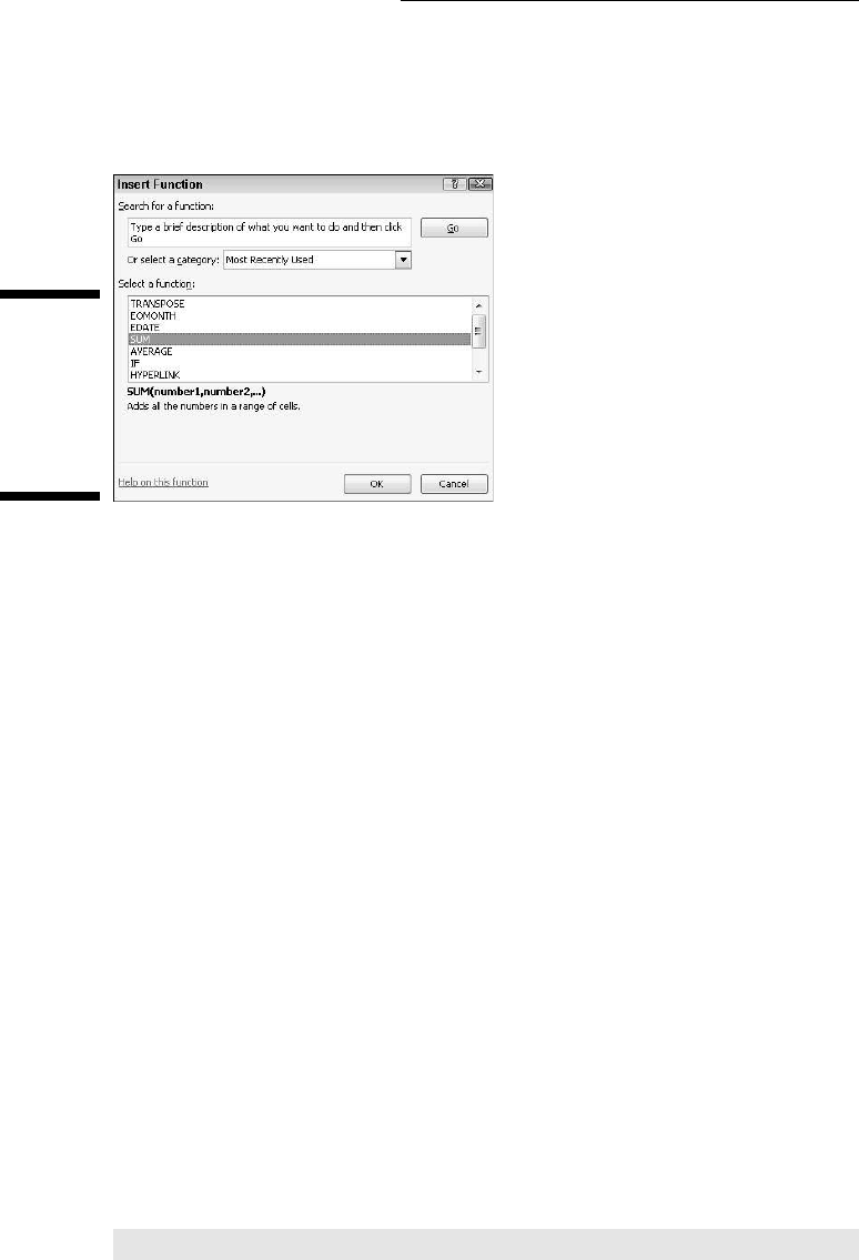
82
Part I: Getting In on the Ground Floor
can get loads of help in completing the argument text boxes in the Function
Arguments dialog box by clicking the Help on This Function link in the lower-
left corner.
Figure 2-15:
Select the
function you
want to use
in the Insert
Function
dialog box.
The Insert Function dialog box contains three boxes: a Search for a Function
text box, an Or Select a Category drop-down list box, and a Select a Function
list box. When you open the Insert Function dialog box, Excel automatically
selects Most Recently Used as the category in the Select a Category drop-
down list box and displays the functions you usually use in the Select a
Function list box.
If your function isn’t among the most recently used, you must then select the
appropriate category of your function in the Select a Category drop-down
list box. If you don’t know the category, you must search for the function by
typing a description of its purpose in the Search for a Function text box and
then press Enter or click the Go button. For example, to locate all the Excel
functions that total values, you enter total in the Search for Function list box
and click the Go button. Excel then displays its list of recommended func-
tions for calculating totals in the Select a Function list box. You can peruse
the recommended functions by selecting each one. While you select each
function in this list, the Insert Function dialog box shows you the required
arguments followed by a description, at the bottom of the dialog box, of what
the function does.
After you locate and select the function that you want to use, click the OK
button to insert the function into the current cell and open the Function
Arguments dialog box. This dialog box displays the required arguments for
the function along with any that are optional. For example, suppose that you
select the SUM function (the crown jewel of the Most Recently Used function
category) in the Select a Function list box and then click OK. As soon as you
do, the program inserts
SUM()
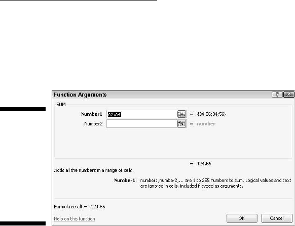
83
Chapter 2: Creating a Spreadsheet from Scratch
in the current cell and on the Formula bar (following the equal sign), and the
Function Arguments dialog box showing the SUM arguments appears on the
screen (as shown in Figure 2-16). This is where you add the arguments for the
SUM function.
Figure 2-16:
Specify the
arguments
to use in the
selected
function in
the Function
Arguments
dialog box.
As shown in Figure 2-16, you can sum up to 255 numbers in the Function
Arguments dialog box. What’s not obvious, however (there’s always some
trick, huh?), is that these numbers don’t have to be in single cells. In fact,
most of the time you’ll be selecting a whole slew of numbers in nearby cells
(in a multiple cell selection — that range thing) that you want to total.
To select your first number argument in the dialog box, you click the cell (or
drag through the block of cells) in the worksheet while the insertion point
is in the Number1 text box. Excel then displays the cell address (or range
address) in the Number1 text box while, at the same time, showing the value
in the cell (or values, if you select a bunch of cells) in the box to the right.
Excel displays the total near the bottom of the Function Arguments dialog
box after the words Formula result=.
When selecting cells, you can minimize this arguments dialog box to just the
contents of the Number1 text box by dragging the cell pointer through the
cells to sum in the worksheet. After you minimize the arguments dialog box
while selecting the cells for the first argument, you can then expand it again
by releasing the mouse button.
You can also reduce the dialog box to the Number1 argument text box by
clicking the Minimize Dialog Box button on the right of the text box, selecting
the cells, and then clicking the Maximize Dialog Box button (the only button
displayed on the far right) or by pressing the Esc key. Instead of minimizing
the dialog box, you can also temporarily move it out of the way by clicking
on any part and then dragging the dialog box to its new destination on the
screen.

84
Part I: Getting In on the Ground Floor
If you’re adding more than one cell (or bunch of cells) in a worksheet, press
the Tab key or click the Number2 text box to move the insertion point to that
text box. (Excel responds by extending the argument list with a Number3 text
box.) Here is where you specify the second cell (or cell range) to add to the
one now showing in the Number1 text box. After you click the cell or drag
through the second cell range, the program displays the cell address(es), the
numbers in the cell(s) to the right, and the running total near the bottom of
the Function Arguments dialog box after Formula result= (as shown in Figure
2-16). You can minimize the entire Function Arguments dialog box down to
just the contents of the argument text box you’re dealing with (Number2,
Number3, and so on) by clicking its particular Minimize Dialog Box button if
the dialog box obscures the cells that you need to select.
When you finish pointing out the cells or bunch of cells to sum, click the OK
button to close the Function Arguments dialog box and put the SUM function
in the current cell.
Editing a function with the
Insert Function button
You can also use the Insert Function button to edit formulas that contain
functions right from the Formula bar. Select the cell with the formula and
function to edit before you click the Insert Function button (the one sport-
ing the fx that appears immediately in front of the current cell entry on the
Formula bar).
As soon as you click the Insert Function button, Excel opens the Function
Arguments dialog box where you can edit its arguments. To edit just the
arguments of a function, select the cell references in the appropriate argu-
ment’s text box (marked Number1, Number2, Number3, and so on) and then
make whatever changes are required to the cell addresses or select a new
range of cells.
Excel automatically adds any cell or cell range that you highlight in the work-
sheet to the current argument. If you want to replace the current argument,
you need to highlight it and remove its cell addresses by pressing the Delete
key before you highlight the new cell or cell range to use as the argument.
(Remember that you can always minimize this dialog box or move it to a new
location if it obscures the cells you need to select.)
When you finish editing the function, press Enter or click the OK button in
the Function Arguments dialog box to put it away and update the formula in
the worksheet.

85
Chapter 2: Creating a Spreadsheet from Scratch
I’d be totally lost without AutoSum
Before leaving this fascinating discussion on entering functions, I want you to
get to the AutoSum tool in the Editing group on the Home tab of the Ribbon.
Look for the Greek sigma (Σ) symbol. This little tool is worth its weight in
gold. In addition to entering the SUM, AVERAGE, COUNT, MAX, or MIN functions,
it also selects the most likely range of cells in the current column or row that
you want to use as the function’s argument and then automatically enters
them as the function’s argument. Nine times out of ten, Excel selects (with
the marquee or moving dotted line) the correct cell range to total, average,
count, and so forth. For that tenth case, you can manually correct the range
by simply dragging the cell pointer through the block of cells to sum.
Simply click the AutoSum button on the Home tab when you want to insert
the SUM function into the current cell. If you want to use this button to insert
another function, such as AVERAGE, COUNT, MAX, or MIN, you need to click its
drop-down button and select the name of the desired function on its pop-up
menu (click Count Numbers on the menu to insert the COUNT function). If you
select the More Functions command on this menu, Excel opens the Insert
Function dialog box as though you had clicked the fx button on the
Formula bar.
In Figure 2-17, check out how to use the AutoSum tool to total the sales of
Jack Sprat Diet Centers in row 3. Position the cell pointer in cell E3 where the
first-quarter total is to appear and then click the AutoSum tool. Excel inserts
SUM (equal sign and all) onto the Formula bar; places a marquee around the
cells B3, C3, and D3; and uses the cell range B3:D3 as the argument of the
SUM function.
Figure 2-17:
To total
Jack Sprat
Diet Centers
first quar-
ter sales
for row 3,
click the
AutoSum
button in
cell E3 and
press Enter.
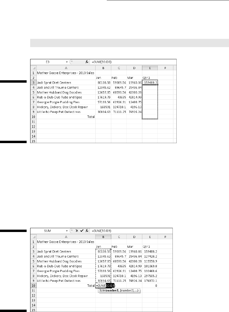
86
Part I: Getting In on the Ground Floor
Now look at the worksheet after you insert the function in cell E3 (see Figure
2-18). The calculated total appears in cell E3 while the following SUM function
formula appears in the Formula bar:
=SUM(B3:D3)
Figure 2-18:
The work-
sheet with
the first
quarter
totals cal-
culated with
AutoSum.
After entering the function to total the sales of Jack Sprat Diet Centers, you
can copy this formula to total sales for the rest of the companies by dragging
the fill handle down column E until the cell range E3:E10 is highlighted.
Look at Figure 2-19 to see how you can use the AutoSum tool to total the
January sales for all the Mother Goose Enterprises in column B. Position the
cell pointer in cell B10 where you want the total to appear. Click the AutoSum
tool, and Excel places the marquee around cells B3 through B9 and correctly
enters the cell range B3:B9 as the argument of the SUM function.
Figure 2-19:
Click the
AutoSum
button in
cell B10 and
press Enter
to total the
January
sales for all
companies
in column B.
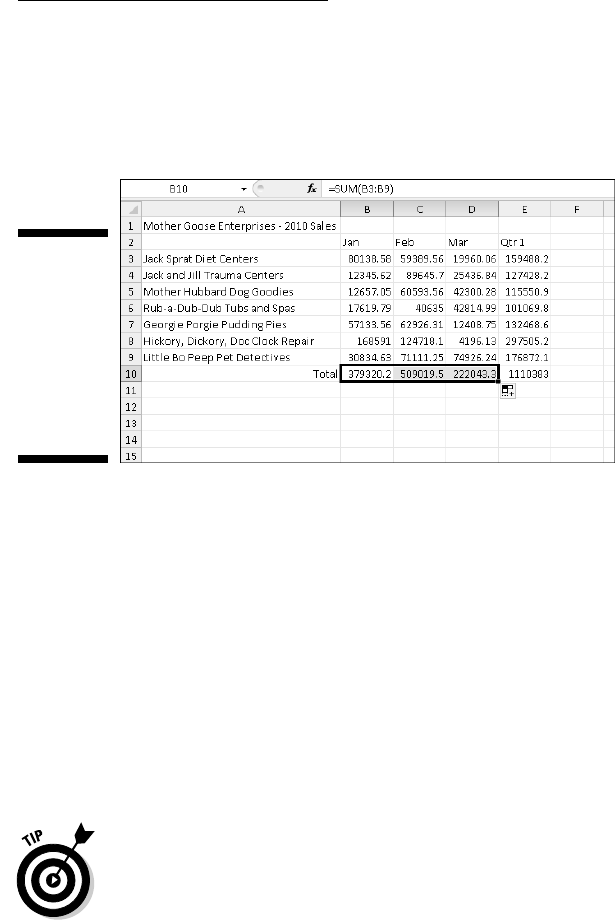
87
Chapter 2: Creating a Spreadsheet from Scratch
In Figure 2-20, you see the worksheet after inserting the function in cell B10
and using the AutoFill feature to copy the formula to cells C10 and D10 to the
right. (To use AutoFill, drag the fill handle through the cells to the right until
you reach cell D10. Release the mouse button.)
Figure 2-20:
The work-
sheet after
copying
the SUM
function
formulas
using the fill
handle.
Making Sure That the Data
Is Safe and Sound
All the work you do in any of the worksheets in your workbook is at risk
until you save the workbook as a disk file, normally on your computer’s hard
drive. Should you lose power or should your computer crash for any reason
before you save the workbook, you’re out of luck. You have to re-create each
keystroke — a painful task, made all the worse because it’s so unnecessary.
To avoid this unpleasantness altogether, adopt this motto: Save your work
any time that you enter more information than you could possibly bear to
lose.
To encourage frequent saving on your part, Excel even provides you with a
Save button on the Quick Access toolbar (the one with the picture of a 3¼ ”
floppy disk, the very first on the toolbar). You don’t even have to take the
time and trouble to choose the Save command from the File pull-down menu
(opened by choosing File) or even press Ctrl+S; you can simply click this tool
whenever you want to save new work on disk.
When you click the Save button, press Ctrl+S, or choose File➪Save for the
first time, Excel displays the Save As dialog box. Use this dialog box to
replace the temporary document name (Book1, Book2, and so forth) with a
more descriptive filename in the File Name text box, select a new file format
in the Save As Type drop-down list box, and select a new drive and folder
before you save the workbook as a disk file.
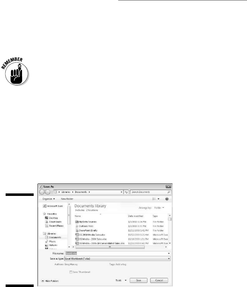
88
Part I: Getting In on the Ground Floor
When you finish making changes in the Save As dialog box, click the Save
button or press Enter to have Excel 2010 save your work. When Excel saves
your workbook file, the program saves all the information in every worksheet
in your workbook (including the last position of the cell cursor) in the desig-
nated folder and drive.
You don’t have to fool with the Save As dialog box again unless you want to
rename the workbook or save a copy of it in a different folder. If you want to
do these things, you must choose File➪Save As or press Alt+FA to choose the
Save As command rather than clicking the Save button on the Quick Access
toolbar or pressing Ctrl+S.
The Save As dialog box in Windows 7
and Windows Vista
Figure 2-21 shows you the Save As dialog box as it appears in Excel 2010
when running the program under Windows 7. Here, you can replace the tem-
porary filename (Book1, Book2, and so on) with a more descriptive name by
clicking the File Name text box and typing in the new name (up to 255 charac-
ters total, including spaces).
Figure 2-21:
The Save As
dialog box
enables you
to select the
filename
and folder
for the new
workbook
file as well
as add tags
to it.
To select a new folder in which to save the new workbook file, follow these
steps:
1. In the Navigation Pane, click the name of the folder in the Favorites,
Libraries, Computer, or Network section in which you want to save
the workbook file.

89
Chapter 2: Creating a Spreadsheet from Scratch
2. To save the workbook file within a subfolder of one of the folders now
displayed in the main pane of the Save As dialog box, double-click its
folder icon to open it up.
3. (Optional) If you want to save the workbook file inside a new sub-
folder within the folder currently open in the Save As dialog box,
click the New Folder button on the toolbar, replace the suggested New
Folder name by typing the actual name of the folder, and then press
Enter.
4. Click the Save button to save the file in the selected folder.
When the Save As dialog box is expanded by clicking the Browse Folders
button, you can modify the authors or add tags to the new workbook file by
clicking the Add an Author or Add a Tag text boxes. You can then use this
information later when searching for the workbook. (See Chapter 4 for details
on searching.)
The Save As dialog box in Windows XP
The Windows XP version of the Save As dialog box contains a bunch of large
buttons that appear on the left side of the dialog box: My Recent Documents,
Desktop, My Documents, My Computer, and My Network Places. Use these but-
tons to select the following folders in which to save your new workbook file:
✓ Click the My Recent Documents button to save your workbook in the
Recent folder. The Recent folder resides in this hierarchy: Windows
folder (on your hard drive)\Application Data folder\Microsoft folder\
Office folder\Recent folder.
✓ Click the Desktop button to save your workbook on your computer’s
desktop.
✓ Click the My Documents button to save your workbook in the My
Documents folder.
✓ Click the My Computer button to save your workbook on one of the
disks on your computer or in your own or a shared documents folder on
your hard drive.
✓ Click the My Network Places button to save your workbook in one of the
folders on your company’s network.
To save your workbook in a new subfolder within the folder open in the Save
As dialog box, click the Create New Folder button on the toolbar (or press
Alt+4) and then type the name for the folder in the New Folder dialog box
before you click OK.

90
Part I: Getting In on the Ground Floor
Changing the default file location
Whenever you open the Save As dialog box to save a new workbook file,
Excel 2010 automatically selects the folder listed in the Default File Location
text box on the Save tab of the Excel Options dialog box (File➪Options➪Save
or Alt+FIS).
When you first start using Excel, the default folder is either the My
Documents (Windows XP) or the Documents folder (Windows 7 and Windows
Vista) under your user name on your hard drive. For example, the directory
path of the default folder where Excel 2010 automatically saves new work-
book files on my computer running Windows XP is
C:\Documents and Settings\Greg\My Documents
However, the directory path of the default folder where Excel 2010 automati-
cally saves new workbook files on my other computer running Windows 7 is
C:\Users\Greg\Documents
The very generic My Documents or Documents folder may not be the places
on your hard drive where you want all the new workbooks you create auto-
matically saved. To change the default file location to another folder on your
computer, follow these steps:
1. Choose File➪Options➪Save or press Alt+FIS to open the Save tab of
the Excel Options dialog box.
The Default File Location text box displays the directory path to the cur-
rent default folder.
2. Click the Default File Location text box.
To edit part of the path (such as the My Documents or Documents folder
name after your user name), click the mouse pointer at that place in the
path to set the insertion point.
3. Edit the existing path or replace it with the path to another folder in
which you want all future workbooks to save to automatically.
4. Click OK to close the Excel Options dialog box.
The difference between the XLSX
and XLS file format
Excel 2010 supports the use of the XML-based file format first introduced in
Excel 2007 (which Microsoft officially calls the Microsoft Office Open XML
format). This default file format is touted as being more efficient in saving

91
Chapter 2: Creating a Spreadsheet from Scratch
data resulting in smaller file size and offering superior integration with exter-
nal data sources (especially, when these resources are Web-based ones sup-
porting XML files). This XML-based file format carries the filename extension
.xlsx and is the file format in which Excel automatically saves any new
workbook you create.
The only problem with this newfangled XML-based file format is that it can’t
be opened by earlier Excel versions (before Excel 2007). Therefore, if someone
who needs to work with the workbook you’ve just created isn’t using Excel
2007 or hasn’t yet upgraded to Excel 2010, you need to save the new workbook
in the earlier file format used in Excel versions 97 through 2003 with the old
.xls filename extension.
To do this, click the Save As Type drop-down button in the Save As dialog
box and then click Excel 97-2003 Workbook (*.xls) on the drop-down menu.
(If you work in an office where all workbooks must be backwardly compatible
with earlier versions, see “Dealing with the new Excel file formats” in Chapter
1 for a tip on making the Excel 97-2003 workbook file format the default
format for Excel 2010.)
Filename extensions, such as .xlsx and .xls, do not appear as part of the
filename (even though they are appended) in the File Name text box in the
Excel Save As dialog box unless you’ve specifically changed Windows’ folder
options to show them. To make this change, open the Folder Options dialog
box in Windows Explorer and then deselect the Hide Extensions for Known
File Types check box on the View tab. To open the Folder Options dialog box,
select Tools➪Options on the Explorer window’s pull-down menus in Windows
XP or click the Organize button and then select Folder and Search Options on
its drop-down menu in Windows 7 and Windows Vista.
Excel 2010 also supports a special binary file format called Excel Binary
Workbook that carries the .xlsb filename extension. Select this binary format
for huge spreadsheets that you create that have to be compatible with earlier
versions of Excel.
Saving the Workbook as a PDF File
The PDF (Portable Document File) file format developed by Adobe Systems
Incorporated enables people to open up and print documents without access
to the original programs with which the documents were created.
Excel 2010 enables you to save your workbook files directly in this special
PDF file format. You can readily share your Excel 2010 workbooks with users
who don’t have Excel installed on their computers by saving them as PDF
files. All they need to open and print the PDF copy of the workbook file is the
free Adobe Reader software (which they can download from the Adobe Web
site at www.adobe.com).

92
Part I: Getting In on the Ground Floor
To save your workbook as a PDF file, you simply select the PDF option on the
Save as Type drop-down list in the Save As dialog box. Excel then adds PDF-
specific options to the bottom of the Save As dialog box, with the Standard
(Publishing Online and Printing) button under the Optimize For heading and
the Open File after Publishing check box selected.
If you want to make the resulting PDF file as small as possible (because your
worksheet is so large), click the Minimum Size (Publishing Online) button
under the Optimize For heading. If you want to change which parts of the
workbook are saved in the resulting PDF (Excel automatically saves all ranges
in the active worksheet of the workbook), click the Options button directly
beneath the Minimum Size (Publishing Online) option and make the appropri-
ate changes in the Options dialog box before you click OK.
If you don’t need to edit the filename (Excel automatically appends .pdf to
the current filename) or the folder location in the Save As dialog box, simply
click the Save button. Excel then saves a copy of the workbook in a PDF file
format and, provided you don’t deselect the Open File after Publishing check
box, automatically opens the workbook for your inspection in Adobe Reader.
After viewing the PDF version in Adobe Reader, you can then return to your
worksheet in Excel by clicking Reader’s Close button (or pressing Alt+F4).
If you create an Excel 2010 workbook that incorporates new features not sup-
ported in earlier versions of Excel, instead of saving the workbook as an .xls
file, thereby losing all of its 2010 enhancements, consider saving it as a PDF
file. That way, co-workers still using pre-2010 Excel versions can still access
the data in all its glory via Adobe Reader.
Document Recovery to the Rescue
Excel 2010 offers a document recovery feature that can help you in the event
of a computer crash because of a power failure or some sort of operating
system freeze or shutdown. The AutoRecover feature saves your work-
books at regular intervals. In the event of a computer crash, Excel displays a
Document Recovery task pane the next time you start Excel after rebooting
the computer.
When you first start using Excel 2010, the AutoRecover feature is set to
automatically save changes to your workbook (provided that the file has
already been saved) every ten minutes. You can shorten or lengthen this
interval as you see fit. Choose File➪Options➪Save or press Alt+FIS to open
the Excel Options dialog box with the Save tab selected. Use the spinner but-
tons or enter a new automatic save interval into the text box marked Save
AutoRecover Information Every 10 Minutes before clicking OK.

93
Chapter 2: Creating a Spreadsheet from Scratch
After re-launching Excel 2010 after a computer crash that prevents you from
saving your workbook file, the program opens with the Document Recovery
task pane on the left side of the screen. This Document Recovery task pane
shows the available versions of the workbook files that were open at the time
of the computer crash. The original version of the workbook file is identified,
including when it was saved, as is the recovered version of the file (display-
ing an .xlsb file extension) and when it was saved.
To open the recovered version of a workbook (to see how much of the work
it contains that was unsaved at the time of the crash), position the mouse
pointer over the AutoRecover version, click its drop-down menu button, and
then click Open. After you open the recovered version, you can then (if you
choose) save its changes by clicking the Save button on the Quick Access
toolbar or by choosing File➪Save.
To save the recovered version of a workbook without bothering to first open
it, place your mouse over the recovered version in the task pane, click its
drop-down button, and then choose Save As. To abandon the recovered ver-
sion permanently (leaving you with only the data in the original version),
click the Close button at the bottom of the Document Recovery task pane.
When you click the Close button, an alert dialog box appears, giving you the
chance to retain the recovered versions of the file for later viewing. To retain
the files for later viewing, select the Yes (I Want to View These Files Later)
radio button before clicking OK. To retain only the original versions of the
files shown in the task pane, select the No (Remove These Files. I Have Saved
the Files I Need) radio button instead.
The AutoRecover features only work on Excel workbooks that you’ve saved
at least one time (as explained in the earlier section “Making Sure That the
Data Is Safe and Sound”). In other words, if you build a new workbook and
don’t bother to save and rename it prior to experiencing a computer crash,
the AutoRecover feature will not bring back any part of it. For this reason, it is
very important that you get into the habit of saving new workbooks with the
Save button on the Quick Access toolbar very shortly after beginning to work
on its worksheets. Or use the trusty keyboard shortcut Ctrl+S.

94
Part I: Getting In on the Ground Floor

Part II
Editing without
Tears

In this part . . .
T
he business world wouldn’t be half-bad if it weren’t
for the fact that right around the time you master
your job, somebody goes and changes it on you. When
your life must always be flexible, changing gears and
“going with the flow” can really grate on a person! The sad
truth is that a big part of the work you do with Excel 2010
is changing the stuff you slaved so hard to enter into the
spreadsheet in the first place.
In Part II, I break down this editing stuff into three phases:
formatting the raw data; rearranging the formatted data or
in some cases deleting it; and spitting out the final format-
ted and edited data in printed form. Take it from me, after
you know your way around editing your spreadsheets (as
presented in this part of the book), you’re more than half-
way home with Excel 2010.

Chapter 3
Making It All Look Pretty
In This Chapter
▶ Selecting the cells to format
▶ Formatting data tables with the Format as Table command button
▶ Using various number formats on cells containing values
▶ Adjusting column width and row height in a worksheet
▶ Hiding columns and rows in a worksheet
▶ Formatting cell ranges from the Home tab of the Ribbon
▶ Formatting cell ranges using Styles and the Format Painter
▶ Formatting cells under certain conditions
I
n spreadsheet programs like Excel, you normally don’t worry about how
the stuff looks until after you enter all the data in the worksheets of your
workbook and save it all safe and sound (see Chapters 1 and 2). Only then do
you pretty up the information so that it’s clearer and easy to read.
After you decide on the types of formatting that you want to apply to a por-
tion of the worksheet, you can select all the cells to beautify and then click
the appropriate tool or choose the menu command to apply those formats to
the cells. However, before you discover all the fabulous formatting features
you can use to dress up cells, you need to know how to pick the group of
cells that you want to apply the formatting to — that is, selecting the cells or,
alternately, making a cell selection.
Be aware, also, that entering data into a cell and formatting that data are
two completely different things in Excel. Because they’re separate, you can
change the entry in a formatted cell, and new entries assume the cell’s for-
matting. This enables you to format blank cells in a worksheet, knowing that
when you get around to making entries in those cells, those entries automati-
cally assume the formatting you assign to those cells.
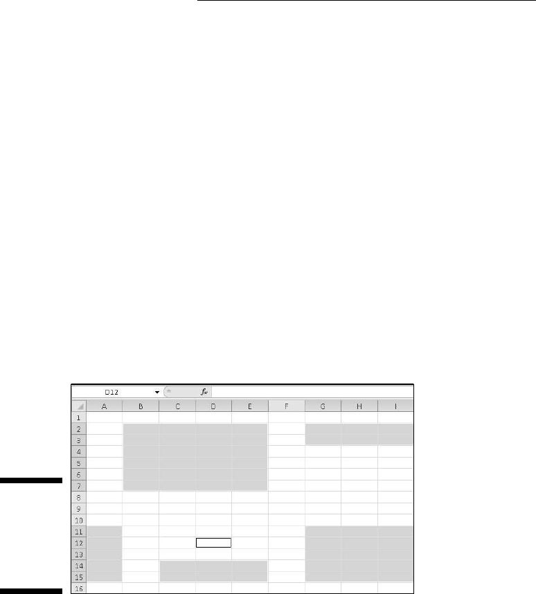
98
Part II: Editing without Tears
Choosing a Select Group of Cells
Given the monotonously rectangular nature of the worksheet and its compo-
nents, it shouldn’t come as a surprise to find that all the cell selections you
make in the worksheet have the same kind of cubist feel to them. After all,
worksheets are just blocks of cells of varying numbers of columns and rows.
A cell selection (or cell range) is whatever collection of neighboring cells you
choose to format or edit. The smallest possible cell selection in a worksheet
is just one cell: the so-called active cell. The cell with the cell cursor is really
just a single cell selection. The largest possible cell selection in a worksheet
is all the cells in that worksheet (the whole enchilada, so to speak). Most
of the cell selections you need for formatting a worksheet will probably fall
somewhere in between, consisting of cells in several adjacent columns and
rows.
Excel shows a cell selection in the worksheet by highlighting in color the
entire block of cells within the extended cell cursor except for the active cell
that keeps its original color. (Figure 3-1 shows several cell selections of differ-
ent sizes and shapes.)
Figure 3-1:
Several cell
selections
of various
shapes and
sizes.
In Excel, you can select more than one cell range at a time (a phenomenon
somewhat ingloriously called a noncontiguous or nonadjacent selection). In
fact, although Figure 3-1 appears to contain several cell selections, it’s really
just one big, nonadjacent cell selection with cell D12 (the active one) as the
cell that was selected last.

99
Chapter 3: Making It All Look Pretty
Point-and-click cell selections
The mouse is a natural for selecting a range of cells. Just position the mouse
pointer (in its thick, white cross form) on the first cell and then click and
drag in the direction that you want to extend the selection.
✓ To extend the cell selection to columns to the right, drag your mouse to
the right, highlighting neighboring cells as you go.
✓ To extend the selection to rows to the bottom, drag your mouse down.
✓ To extend the selection down and to the right at the same time, drag
your mouse diagonally toward the cell in the lower-right corner of the
block you’re highlighting.
Shifty cell selections
To speed up the old cell-selection procedure, you can use the Shift+click
method, which goes as follows:
1. Click the first cell in the selection.
This selects that cell.
2. Position the mouse pointer in the last cell in the selection.
This is kitty-corner from the first cell in your selected rectangular block.
3. Press the Shift key and hold it down while you click the mouse button
again.
When you click the mouse button the second time, Excel selects all the
cells in the columns and rows between the first cell and last cell.
The Shift key works with the mouse like an extend key to extend a selection
from the first object you select through to, and including, the second object
you select. See the section “Extend that cell selection,” later in this chapter.
Using the Shift key enables you to select the first and last cells, as well as all
the intervening cells in a worksheet or all the document names in a dialog list
box.
If, when making a cell selection with the mouse, you notice that you include
the wrong cells before you release the mouse button, you can deselect the
cells and resize the selection by moving the pointer in the opposite direction.
If you already released the mouse button, click the first cell in the highlighted
range to select just that cell (and deselect all the others) and then start the
whole selection process again.

100
Part II: Editing without Tears
Nonadjacent cell selections
To select a nonadjacent cell selection made up of more than one non-touching
block of cells, drag through the first cell range and release the mouse button.
Then hold down the Ctrl key while you click the first cell of the second range
and drag the pointer through the cells in this range. As long as you hold
down Ctrl while you select the subsequent ranges, Excel doesn’t deselect any
of the previously selected cell ranges.
The Ctrl key works with the mouse like an add key to include non-neighboring
objects in Excel. See the section “Nonadjacent cell selections with the key-
board,” later in this chapter. By using the Ctrl key, you can add to the selec-
tion of cells in a worksheet or to the document names in a dialog list box
without having to deselect those already selected.
Going for the “big” cell selections
You can select the cells in entire columns or rows or even all the cells in the
worksheet by applying the following clicking-and-dragging techniques to the
worksheet frame:
✓ To select every single cell in a particular column, click its column letter
on the frame at the top of the worksheet document window.
✓ To select every cell in a particular row, click its row number on the
frame at the left edge of the document window.
✓ To select a range of entire columns or rows, drag through the column
letters or row numbers on the frame surrounding the workbook.
✓ To select more than entire columns or rows that are not right next to
each other (that old noncontiguous stuff, again), press and hold down
the Ctrl key while you click the column letters or row numbers of the
columns and rows that you want to add to the selection.
✓ To select every cell in the worksheet, press Ctrl+A or click the Select All
button, which is the button with the triangle pointing downward on the
diagonal (reminding me of the corner of a dog-eared book page). It’s in the
upper-left corner of the workbook frame, formed by the intersection of the
row with the column letters and the column with the row numbers.
Selecting the cells in a table of data, courtesy of AutoSelect
Excel provides a quick way (called AutoSelect) to select all the cells in a table
of data entered as a solid block. To use AutoSelect, simply follow these steps:
1. Click the first cell of the table to select it.
This is the cell in the table’s upper-left corner.
2. Hold down the Shift key while you double-click the right or bottom
edge of the selected cell with the arrowhead mouse pointer. (See
Figure 3-2.)
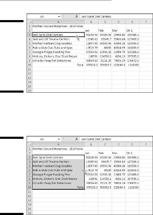
101
Chapter 3: Making It All Look Pretty
Figure 3-2:
Position
the mouse
pointer on
the first
cell’s bot-
tom edge
to select all
cells of the
table’s first
column.
Double-clicking the bottom edge of the cell causes the cell selection to
expand to the cell in the last row of the first column (as shown in Figure
3-3). If you double-click the right edge of the cell, the cell selection
expands to the cell in the last column of the first row.
Figure 3-3:
Hold down
Shift while
you double-
click the
bottom
edge of the
first cell to
extend the
selection
down the
column.
3a. Double-click somewhere on the right edge of the cell selection (refer
to Figure 3-3) if the cell selection now consists of the first column of
the table.
This selects all the remaining rows of the table of data (as shown in
Figure 3-4).
3b. Double-click somewhere on the bottom edge of the current cell selec-
tion if the cell selection now consists of the first row of the table.
This selects all the remaining rows in the table.
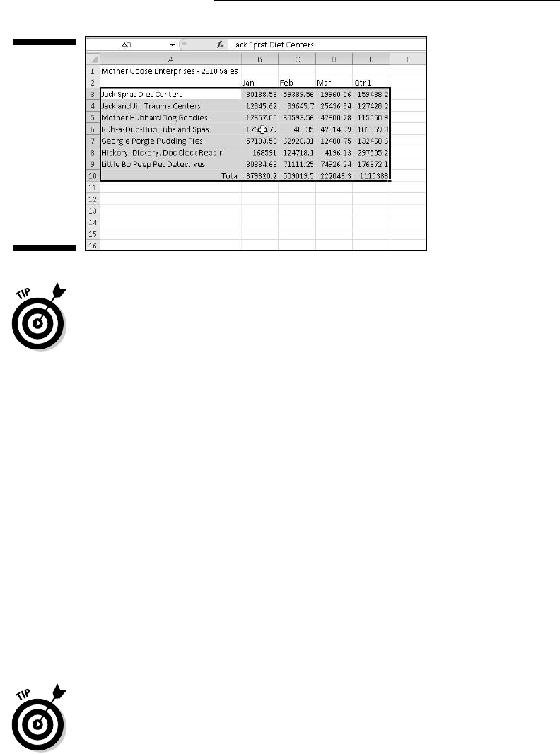
102
Part II: Editing without Tears
Figure 3-4:
Hold down
Shift as you
double-click
the right
edge of
the current
selection
to extend it
across the
rows of the
table.
Although the preceding steps may lead you to believe that you have to select
the first cell of the table when you use AutoSelect, you can actually select any
of the cells in the four corners of the table. Then, when expanding the cell
selection in the table with the Shift key depressed, you can choose whatever
direction you like to either select the first or last row of the table or the first
or last column. (Choose left, by clicking the left edge; right, by clicking the
right edge; up, by clicking the top edge; or down, by clicking the bottom edge.)
After expanding the cell selection to include either the first or last row or first
or last column, you need to click whichever edge of that current cell selection
that will expand it to include all the remaining table rows or columns.
Keyboard cell selections
If you’re not keen on using the mouse, you can use the keyboard to select the
cells you want. Sticking with the Shift+click method of selecting cells, the easi-
est way to select cells with the keyboard is to combine the Shift key with other
keystrokes that move the cell cursor. (I list these keystrokes in Chapter 1.)
Start by positioning the cell cursor in the first cell of the selection and then
holding the Shift key while you press the appropriate cell-pointer movement
keys. When you hold the Shift key while you press direction keys — such as
the arrow keys (↑, →, ↓, ←), PgUp, or PgDn — Excel anchors the selection on
the current cell, moves the cell cursor, and highlights cells as it goes.
When making a cell selection this way, you can continue to alter the size and
shape of the cell range with the cell-pointer movement keys as long as you
don’t release the Shift key. After you release the Shift key, pressing any of the
cell-pointer movement keys immediately collapses the selection, reducing it to
just the cell with the cell cursor.

103
Chapter 3: Making It All Look Pretty
Extend that cell selection
If holding the Shift key while you move the cell cursor is too tiring, you can
place Excel in Extend mode by pressing (and promptly releasing) F8 before
you press any cell-pointer movement key. Excel displays the Extend Selection
indicator on the left side of the Status bar — when you see this, the program
will select all the cells that you move the cell cursor through (just as though
you were holding down the Shift key).
After you highlight all the cells you want in the cell range, press F8 again (or
Esc) to turn off Extend mode. The Extend Selection indicator disappears from
the status bar, and then you can once again move the cell cursor with the
keyboard without highlighting everything in your path. In fact, when you first
move the pointer, all previously selected cells are deselected.
AutoSelect keyboard style
For the keyboard equivalent of AutoSelect with the mouse (see the “Selecting
the cells in a table of data, courtesy of AutoSelect” section), you combine
the use of the F8 key (Extend key) or the Shift key with the Ctrl+arrow keys
or End+arrow keys to zip the cell cursor from one end of a block to the other
and merrily select all the cells in that path.
To select an entire table of data with a keyboard version of AutoSelect, follow
these steps:
1. Position the cell cursor in the first cell.
That’s the cell in the upper-left corner of the table.
2. Press F8 (or hold the Shift key) and then press Ctrl+→ to extend the
cell selection to the cells in the columns on the right.
3. Then press Ctrl+↓ to extend the selection to the cells in the rows
below.
The directions in the preceding steps are somewhat arbitrary — you can just
as well press Ctrl+↓ before you press Ctrl+→. Just be sure (if you’re using the
Shift key instead of F8) that you don’t let up on the Shift key until after you
finish performing these two directional maneuvers. Also, if you press F8 to get
the program into Extend mode, don’t forget to press this key again to get out
of Extend mode after the table cells are all selected, or you’ll end up selecting
cells that you don’t want included when you next move the cell cursor.
Nonadjacent cell selections with the keyboard
Selecting more than one cell range is a little more complicated with the key-
board than it is with the mouse. When using the keyboard, you alternate
between anchoring the cell cursor and moving it to select the cell range and

104
Part II: Editing without Tears
unanchoring the cell cursor and repositioning it at the beginning of the next
range. To unanchor the cell cursor so that you can move it into position for
selecting another range, press Shift+F8. This puts you in Add to Selection
mode, in which you can move to the first cell of the next range without select-
ing any more cells. Excel lets you know that the cell cursor is unanchored by
displaying the Add to Selection indicator on the left side of the Status bar.
To select more than one cell range by using the keyboard, follow these gen-
eral steps:
1. Move the cell cursor to the first cell of the first cell range that you
want to select.
2. Press F8 to get into Extend Selection mode.
Move the cell cursor to select all the cells in the first cell range.
Alternatively, hold the Shift key while you move the cell cursor.
3. Press Shift+F8 to switch from Extend Selection mode to Add to
Selection mode.
The Add to Selection indicator appears in the Status bar.
4. Move the cell cursor to the first cell of the next nonadjacent range that
you want to select.
5. Press F8 again to get back into Extend Selection mode and then move
the cell cursor to select all the cells in this new range.
6. If you still have other nonadjacent ranges to select, repeat Steps 3, 4,
and 5 until you select and add all the cell ranges that you want to use.
Cell selections à la Go To
If you want to select a large cell range that would take a long time to select by
pressing various cell-pointer movement keys, use the Go To feature to extend
the range to a far distant cell. All you gotta do is follow this pair of steps:
1. Position the cell cursor in the first cell of the range and then press F8
to anchor the cell cursor and get Excel into Extend Selection mode.
2. Press F5 or Ctrl+G to open the Go To dialog box, type the address of
the last cell in the range (the cell kitty-corner from the first cell), and
then click OK or press Enter.
Because Excel is in Extend Selection mode at the time you use the Go To fea-
ture to jump to another cell, the program not only moves the cell cursor to
the designated cell address but selects all the intervening cells as well. After
selecting the range of cells with the Go To feature, don’t forget to press F8
(the Extend Selection key) again to prevent the program from messing up your
selection by adding more cells the next time you move the cell cursor.
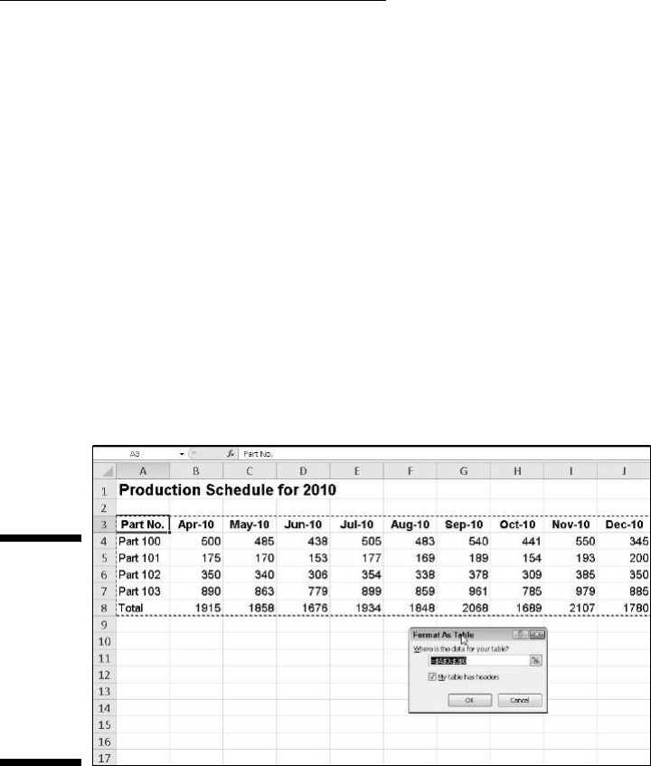
105
Chapter 3: Making It All Look Pretty
Having Fun with the Format
as Table Gallery
Here’s a formatting technique that doesn’t require you to do any prior cell
selecting. (Kinda figures, doesn’t it?) The Format as Table feature is so auto-
matic that the cell cursor just has to be within the table of data prior to you
clicking the Format as Table command button in the Styles group on the
Home tab. Clicking the Format as Table command button opens its rather
extensive Table gallery with the formatting thumbnails divided into three sec-
tions — Light, Medium, and Dark — each of which describes the intensity of
the colors used by its various formats.
As soon as you click one of the table formatting thumbnails in this Table gal-
lery, Excel makes its best guess as to the cell range of the data table to apply
it to (indicated by the marquee around its perimeter) and the Format As
Table dialog box, similar to the one shown in Figure 3-5, appears.
Figure 3-5:
Selecting a
format from
the Table
gallery and
indicating
its range in
the Format
As Table
dialog box.
This dialog box contains a Where Is the Data for Your Table text box that
shows the address of the cell range currently selected by the marquee and a
My Table Has Headers check box.
If Excel does not correctly guess the range of the data table you want to
format, drag through the cell range to adjust the marquee and the range
address in the Where Is the Data for Your Table text box. If your data table
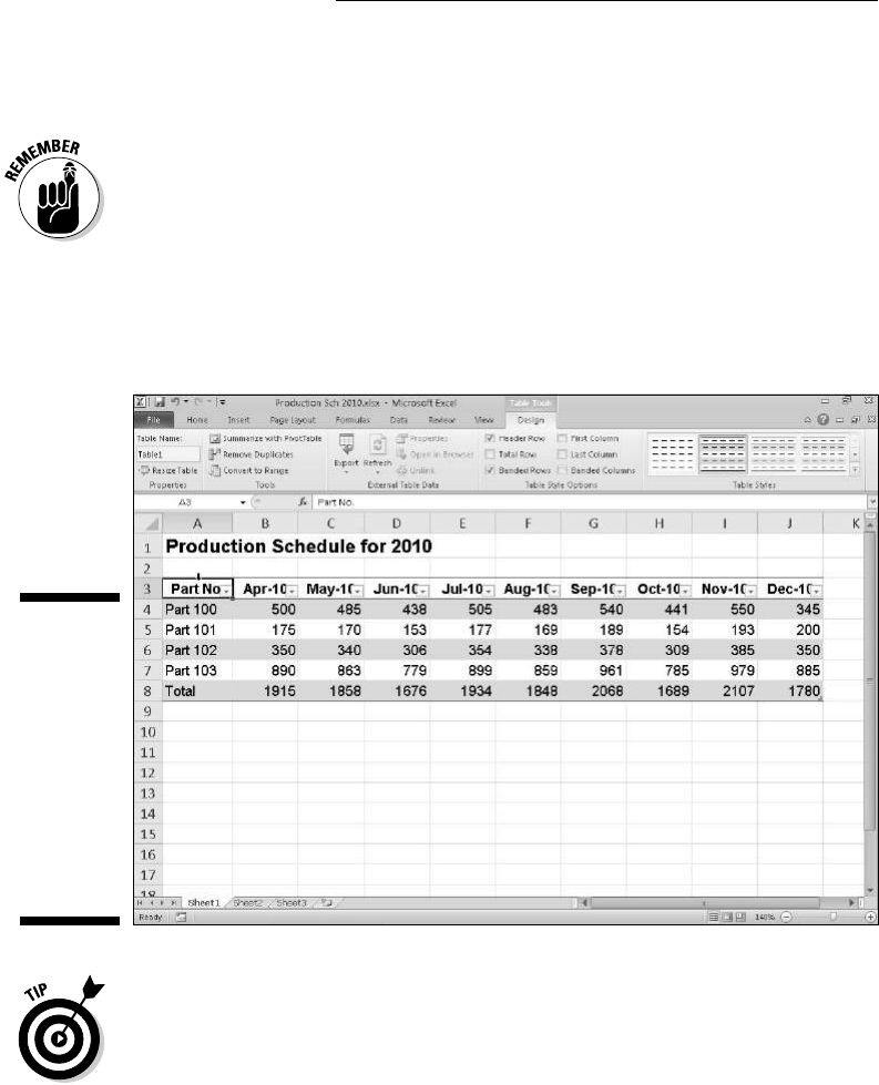
106
Part II: Editing without Tears
doesn’t use column headers or, if the table has them, but you still don’t want
Excel to add Filter drop-down buttons to each column heading, deselect the
My Table Has Headers check box before you click the OK button.
The table formats in the Table gallery are not available if you select multiple
nonadjacent cells before you click the Format as Table command button on
the Home tab.
After you click the OK button in the Format As Table dialog box, Excel
applies the format of the thumbnail you clicked in the gallery to the data
table. Additionally, the Design tab appears under the Table Tools contextual
tab at the end of the Ribbon, as shown in Figure 3-6.
Figure 3-6:
After you
select a
format from
the Table
gallery, the
Design tab
appears
under the
Table Tools
contextual
tab.
The Design tab enables you to use Live Preview to see how your table would
appear. Simply position the mouse pointer over any of the format thumbnails
in the Table Styles group to see the data in your table appear in that table
format. Click the button with the triangle pointing downward to scroll up new
rows of table formats in the Table Styles group and the button with the tri-
angle pointing upward to scroll down rows without opening the Table gallery
and possibly obscuring the actual data table in the Worksheet area. Click the
More button (the one with the horizontal bar above the downward pointing
triangle) to redisplay the Table gallery and then mouse over the thumbnails in
the Light, Medium, and Dark sections to have Live Preview apply them to the
table.

107
Chapter 3: Making It All Look Pretty
In addition to enabling you to select a new format from the Table gallery in
the Table Styles group, the Design tab contains a Table Style Options group
containing a bunch of check boxes that enable you to customize the look of
the selected table format even further:
✓ Header Row to add special formatting and Filter buttons to each of the
column headings in the first row of the table.
✓ Total Row to have Excel add a Total Row to the bottom of the table
that displays the sums of each column that contains values. To apply
another Statistical function to the values in a particular column, click
the cell in that column’s Total Row to display a drop-down list button
and then select the function — Average, Count, Count Numbers, Max,
Min, Sum, StdDev (Standard Deviation), or Var (Variance).
✓ First Column to have Excel display the row headings in the first column
of the table in bold.
✓ Last Column to have Excel display the row headings in the last column
of the table in bold.
✓ Banded Rows to have Excel apply shading to every other row in the
table.
✓ Banded Columns to have Excel apply shading to every other column in
the table.
Whenever you assign a format in the Table gallery to one of the data tables
in your workbook, Excel automatically assigns that table a generic range
name (Table1, Table2, and so on). You can use the Table Name text box in
the Properties group on the Design tab to rename the data table by giving it a
more descriptive range name. (See Chapter 6 for all you need to know about
naming cell ranges.)
When you finish selecting and/or customizing the formatting of your data
table, click a cell outside of the table to remove the Table Tools contextual
tab (with its Design tab) from the Ribbon. If later, you decide that you want to
further experiment with the table’s formatting, click any of the table’s cells to
redisplay the Table Tools’ Design tab at the end of the Ribbon.
Cell Formatting from the Home Tab
Some spreadsheet tables or ranges within them require a lighter touch than
the Format as Table command button offers. For example, you may have a
data table where the only emphasis you want to add is to make the column
headings bold at the top of the table and to underline the row of totals at the
bottom (done by drawing a borderline along the bottom of the cells).

108
Part II: Editing without Tears
The formatting buttons that appear in the Font, Alignment, and Number
groups on the Home tab enable you to accomplish just this kind of targeted
cell formatting. Figures 3-7, 3-8, and 3-9 identify all the formatting buttons in
these three groups on the Home tab. See Table 3-1 for a complete rundown
on how to use each of these formatting buttons.
Figure 3-7:
The Home
tab’s Font
group con-
tains the
tools you
commonly
need when
modifying
the appear-
ance of the
text in a cell
range.
Font Font size Decrease font size
Increase font size
Bold
Underline
Borders
Fill color
Font color
Italic
Figure 3-8:
The Home
tab’s
Alignment
group con-
tains the
tools you
commonly
need when
modifying
the place-
ment of the
text in a cell
range.
Top align
Middle align
Bottom align
Orientation
Wrap text
Left align
Center
Right align
Decrease indent
Increase indent
Merge & center

109
Chapter 3: Making It All Look Pretty
Figure 3-9:
The Home
tab’s
Number
group con-
tains the
tools you
commonly
need when
modifying
the number
format of
the values in
a cell range.
Number format
Accounting number format
Percent style
Comma style
Increase decimal
Decrease decimal
Table 3-1 Formatting Command Buttons in the Font, Alignment,
and Number Groups on the Home Tab
Group Button Name Function
Font
Font Displays a Font drop-down menu from which
you can select a new font for your cell selec-
tion
Font Size Displays a Font Size drop-down menu from
which you can select a new font size for your
cell selection — click the Font Size text box and
enter the desired point size if it doesn’t appear
on the drop-down menu
Increase Font
Size
Increases the size of the font in the cell selec-
tion by one point
Decrease Font
Size
Decreases the size of the font in the cell selec-
tion by one point
Bold Applies boldface to the entries in the cell
selection
Italic Italicizes the entries in the cell selection
Underline Underlines the entries in the cell selection
Borders Displays a Borders drop-down menu from
which you can select a border style for the cell
selection
(continued)

110
Part II: Editing without Tears
Table 3-1 (continued)
Group Button Name Function
Fill Color Displays a Color drop-down palette from which
you can select a new background color for the
cell selection
Font Color Displays a Color drop-down palette from which
you can select a new font color for the cell
selection
Alignment
Align Left Aligns all the entries in the cell selection with
the left edge of their cells
Center Centers all the entries in the cell selection
within their cells
Align Right Aligns all the entries in the cell selection with
the right edge of their cells
Decrease Indent Decreases the margin between entries in the
cell selection and their left cell borders by one
tab stop
Increase Indent Increases the margin between the entries in
the cell selection and their left cell borders by
one tab stop
Top Align Aligns the entries in the cell selection with the
top border of their cells
Middle Align Vertically centers the entries in the cell selec-
tion between the top and bottom borders of
their cells
Bottom Align Aligns the entries in the cell selection with the
bottom border of their cells
Orientation Displays a drop-down menu with options for
changing the angle and direction of the entries
in the cell selection
Wrap Text Wraps the entries in the cell selection that spill
over their right borders onto multiple lines within
the current column width
Merge and
Center
Merges the cell selection into a single cell and
the centers the entry in the first cell between
its new left and right border — click the Merge
and Center drop-down button to display a
menu of options that enable you to merge the
cell selection into a single cell without center-
ing the entries as well as to split up a merged
cell back into its original individual cells

111
Chapter 3: Making It All Look Pretty
Group Button Name Function
Number
Number Format Displays the number format applied to the
active cell in the cell selection — click its drop-
down button to display a menu showing the
active cell in cell selection formatted with all of
Excel’s major number formats
Accounting
Number Format
Formats the cell selection using the Accounting
number format that adds a dollar sign, uses
commas to separate thousands, displays two
decimal places, and encloses negative values
in a closed pair of parentheses — click the
Accounting Number Format’s drop-down
button to display a menu of other major
Currency number formats from which you can
choose
Percent Style Formats the cell selection using the
Percentage number format that multiplies the
values by 100 and adds a percent sign with no
decimal places
Comma Style Formats the cell selection with the Comma
Style number format that uses commas to sep-
arate thousands, displays two decimal places,
and encloses negative values in a closed pair
of parentheses
Increase Decimal Adds a decimal place to the values in the cell
selection
Decrease
Decimal
Removes a decimal place from the values in
the cell selection
Don’t forget about these shortcut keys for quickly adding or removing attri-
butes from the entries in the cell selection: Ctrl+B for toggling on and off bold
in the cell selection, Ctrl+I for toggling on and off italic, and Ctrl+U for toggling
on and off underlining.
Formatting Cells Close to the
Source with the Mini-Toolbar
Excel 2010 makes it easy to apply common formatting changes to a cell selec-
tion right within the Worksheet area thanks to its new mini-toolbar feature,
nicknamed the mini-bar (makes me thirsty just thinking about it!).
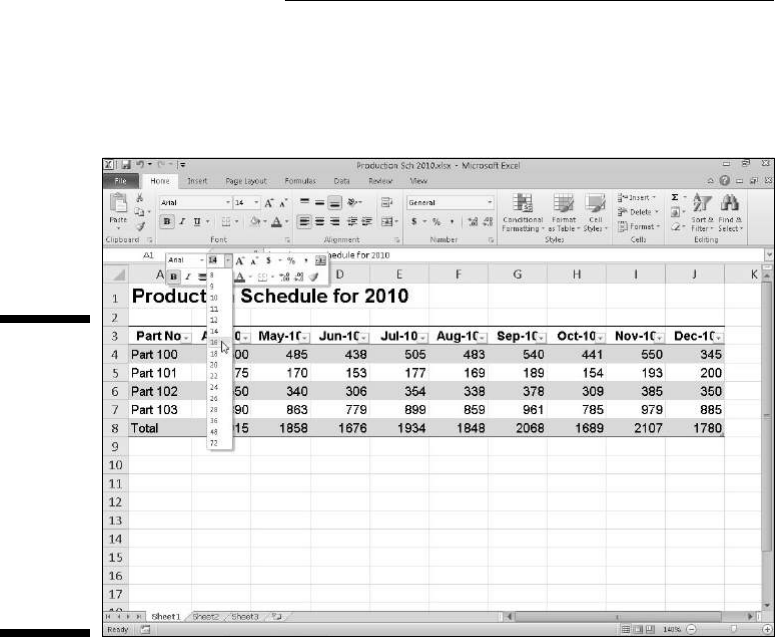
112
Part II: Editing without Tears
To display the mini-bar, select the cells that need formatting and then right-
click somewhere in the cell selection. The mini-toolbar then appears immedi-
ately above the cell selection (see Figure 3-10).
Figure 3-10:
Use the but-
tons on the
mini-toolbar
to apply
common
formatting
changes
to the cell
selection
within the
Worksheet
area.
As you can see in this figure, the mini-toolbar contains most of the buttons
from the Font group of the Home tab (with the exception of the Underline
button). It also contains the Center and Merge & Center buttons from the
Alignment group (see “Altering the Alignment” later in this chapter) and the
Accounting Number Format, Percent Style, Comma Style, Increase Decimal,
and Decrease Decimal buttons from the Number group (see “Getting comfort-
able with the number formats” later in this chapter). Simply click these but-
tons to apply their formatting to the current cell selection.
Additionally, the mini-bar contains the Format Painter button from the
Clipboard group of the Home tab that you can use to copy the formatting
in the active cell to a cell selection you make (see “Fooling Around with the
Format Painter” later in this chapter for details).
Using the Format Cells Dialog Box
Although the command buttons in the Font, Alignment, and Number groups
on the Home tab give you immediate access to the most commonly used

113
Chapter 3: Making It All Look Pretty
formatting commands, they do not represent all of Excel’s formatting com-
mands by any stretch of the imagination.
To have access to all the formatting commands, you need to open the Format
Cells dialog box by doing any of the following:
✓ Click the More Number Formats option at the very bottom of the drop-
down menu attached to the Number Format button
✓ Click the dialog box launcher in the lower right of the Number group
✓ Press Ctrl+1
The Format Cells dialog box that this command calls up contains six tabs:
Number, Alignment, Font, Border, Fill, and Protection. In this chapter, I show
you how to use them all except the Protection tab. For information on that
tab, see Chapter 6.
The keystroke shortcut that opens the Format Cells dialog box — Ctrl+1 — is
one worth knowing. Just press the Ctrl key plus the number 1 key, and not the
function key F1.
Getting comfortable with
the number formats
As I explain in Chapter 2, how you enter values into a worksheet determines
the type of number format that they get. Here are some examples:
✓ If you enter a financial value complete with the dollar sign and two deci-
mal places, Excel assigns a Currency number format to the cell along
with the entry.
✓ If you enter a value representing a percentage as a whole number fol-
lowed by the percent sign without any decimal places, Excel assigns the
cell the Percentage number format that follows this pattern along with
the entry.
✓ If you enter a date (dates are values, too) that follows one of the built-
in Excel number formats, such as 11/06/02 or 06-Nov-02, the program
assigns a Date number format that follows the pattern of the date along
with a special value representing the date.
Although you can format values in this manner as you go along (which is nec-
essary in the case of dates), you don’t have to do it this way. You can always
assign a number format to a group of values before or after you enter them.
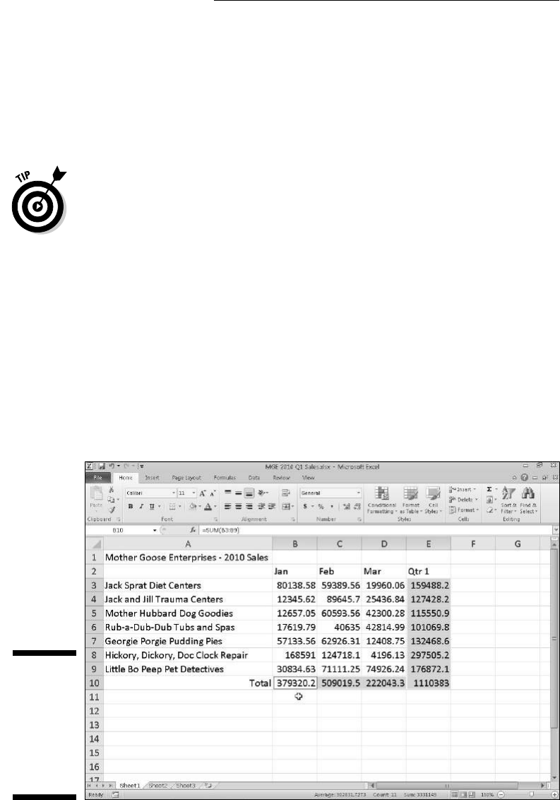
114
Part II: Editing without Tears
Formatting numbers after you enter them is often the most efficient way to go
because it’s just a two-step procedure:
1. Select all the cells containing the values that need dressing up.
2. Select the number format that you want to use from the formatting
command buttons on the Home tab or the options available on the
Number tab in the Format Cells dialog box.
Even if you’re a really, really good typist and prefer to enter each value exactly
as you want it to appear in the worksheet, you still have to resort to using
number formats to make the values that are calculated by formulas match
the others you enter. This is because Excel applies a General number format
(which the Format Cells dialog box defines: “General format cells have no spe-
cific number format.”) to all the values it calculates as well as any you enter
that don’t exactly follow one of the other Excel number formats. The biggest
problem with the General format is that it has the nasty habit of dropping all
leading and trailing zeros from the entries. This makes it very hard to line up
numbers in a column on their decimal points.
You can view this sad state of affairs in Figure 3-11, which is a sample work-
sheet with the first-quarter 2010 sales figures for Mother Goose Enterprises
before any of the values have been formatted. Notice how the numbers in the
monthly sales figures columns zig and zag because they don’t align according
to decimal place. This is the fault of Excel’s General number format; the only
cure is to format the values with a uniform number format.
Figure 3-11:
Numbers
with deci-
mals don’t
align when
you choose
General for-
matting.
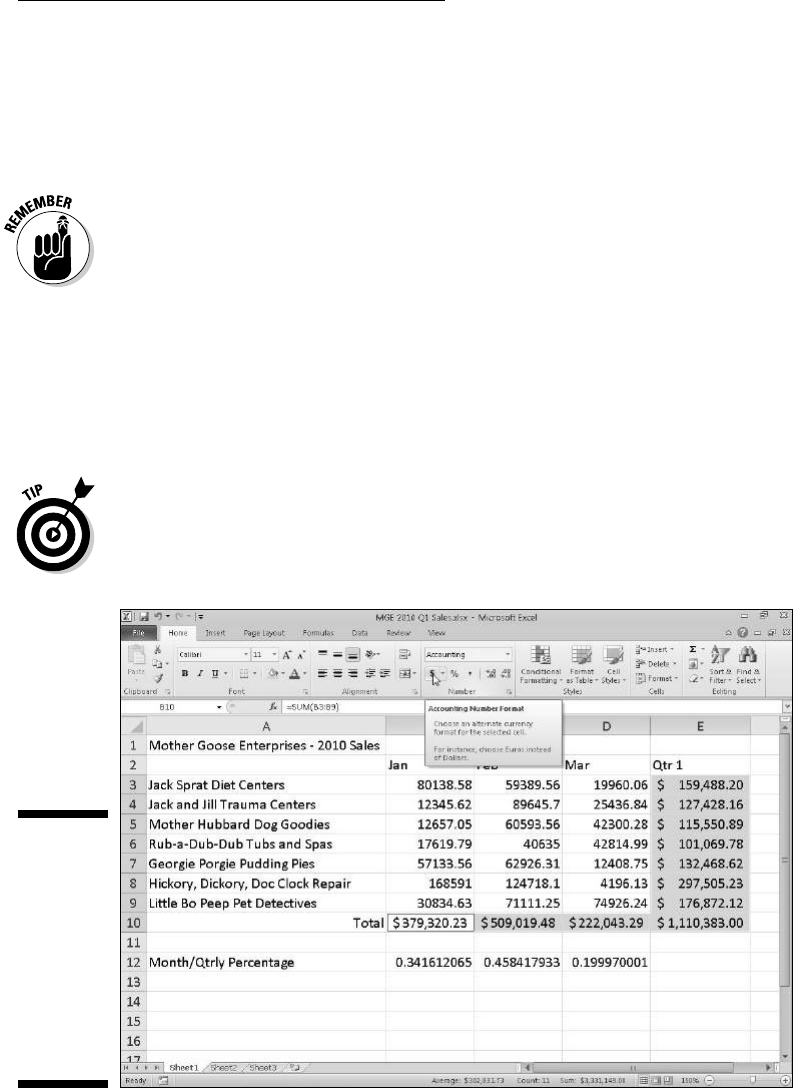
115
Chapter 3: Making It All Look Pretty
Accenting your cells with the Accounting number format
Given the financial nature of most worksheets, you probably use the
Accounting number format more than any other. Applying this format is
easy because you can assign it to the cell selection simply by clicking the
Accounting Number Format button on the Home tab.
The Accounting number format adds a dollar sign, commas between thou-
sands of dollars, and two decimal places to any values in a selected range.
If any of the values in the cell selection are negative, this number format
displays them in parentheses (the way accountants like them). If you want
a minus sign in front of your negative financial values rather than enclosing
them in parentheses, select the Currency format on the Number Format drop-
down menu or on the Number tab of the Format Cells dialog box.
You can see in Figure 3-12 only the cells containing totals are selected (cell
ranges E3:E10 and B10:D10). This cell selection was then formatted with the
Accounting number format by simply clicking its command button (the one
with the $ icon, naturally) in the Number group on the Ribbon’s Home tab.
Although you could put all the figures in the table into the Accounting number
format to line up the decimal points, this would result in a superabundance
of dollar signs in a fairly small table. In this example, I only formatted the
monthly and quarterly totals with the Accounting number format.
Figure 3-12:
The totals in
the Mother
Goose sales
table after
clicking the
Accounting
Number
Format but-
ton on the
Home tab.

116
Part II: Editing without Tears
“Look, Ma, no more format overflow!”
When I apply the Accounting number format to the selection in the cell
ranges of E3:E10 and B10:D10 in the sales table shown in Figure 3-12, Excel
adds dollar signs, commas between the thousands, a decimal point, and two
decimal places to the highlighted values. At the same time, Excel automati-
cally widens columns B, C, D, and E just enough to display all this new for-
matting. In versions of Excel earlier than Excel 2003, you had to widen these
columns yourself, and instead of the perfectly aligned numbers, you were
confronted with columns of #######s in cell ranges E3:E10 and B10:D10. Such
pound signs (where nicely formatted dollar totals should be) serve as over-
flow indicators, declaring that whatever formatting you added to the value in
that cell has added so much to the value’s display that Excel can no longer
display it within the current column width.
Fortunately, Excel eliminates the format overflow indicators when you’re for-
matting the values in your cells by automatically widening the columns. The
only time you’ll ever run across these dreaded #######s in your cells is when
you take it upon yourself to narrow a worksheet column manually (see the
section “Calibrating Columns,” later in this chapter) to the extent that Excel
can no longer display all the characters in its cells with formatted values.
Currying your cells with the Comma Style
The Comma Style format offers a good alternative to the Currency format.
Like Currency, the Comma Style format inserts commas in larger numbers
to separate thousands, hundred thousands, millions, and . . . well, you get
the idea.
This format also displays two decimal places and puts negative values in
parentheses. What it doesn’t display is dollar signs. This makes it perfect
for formatting tables where it’s obvious that you’re dealing with dollars and
cents or for larger values that have nothing to do with money.
The Comma Style format also works well for the bulk of the values in the sample
first-quarter sales worksheet. Check out Figure 3-13 to see this table after I format
the cells containing the monthly sales for all the Mother Goose Enterprises with
the Comma Style format. To do this, select the cell range B3:D9 and click the
Comma Style button — the one with the comma icon (,) — in the Number group
on the Home tab.
Note how, in Figure 3-13, the Comma Style format takes care of the earlier
decimal alignment problem in the quarterly sales figures. Moreover, Comma
Style–formatted monthly sales figures align perfectly with the Currency
format–styled monthly totals in row 10. If you look closely (you may need a
magnifying glass for this one), you see that these formatted values no longer
abut the right edges of their cells; they’ve moved slightly to the left. The gap
on the right between the last digit and the cell border accommodates the
right parenthesis in negative values, ensuring that they, too, align precisely
on the decimal point.
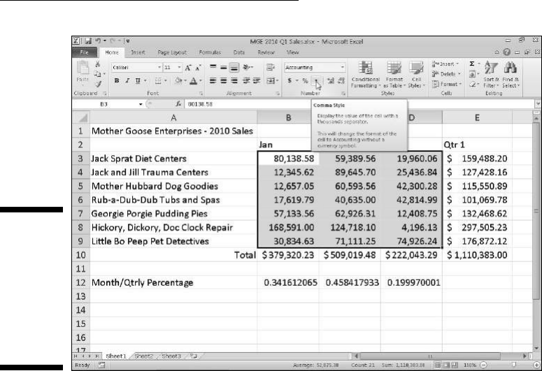
117
Chapter 3: Making It All Look Pretty
Figure 3-13:
Monthly
sales fig-
ures after
formatting
cells with
the Comma
Style num-
ber format.
Playing around with Percent Style
Many worksheets use percentages in the form of interest rates, growth
rates, inflation rates, and so on. To insert a percentage in a cell, type the
percent sign (%) after the number. To indicate an interest rate of 12 percent,
for example, you enter 12% in the cell. When you do this, Excel assigns a
Percentage number format and, at the same time, divides the value by 100
(that’s what makes it a percentage) and places the result in the cell (0.12 in
this example).
Not all percentages in a worksheet are entered by hand in this manner. Some
may be calculated by a formula and returned to their cells as raw decimal
values. In such cases, you should add a Percent format to convert the calcu-
lated decimal values to percentages (done by multiplying the decimal value
by 100 and adding a percent sign).
The sample first-quarter-sales worksheet just happens to have some percent-
ages calculated by formulas in row 12 that need formatting (these formulas
indicate what percentage each monthly total is of the first-quarter total in cell
E10). In Figure 3-14, these values reflect Percent Style formatting. To accom-
plish this feat, you simply select the cells and click the Percent Style button
in the Number group on the Home tab. (Need I point out that it’s the button
with the % symbol?)
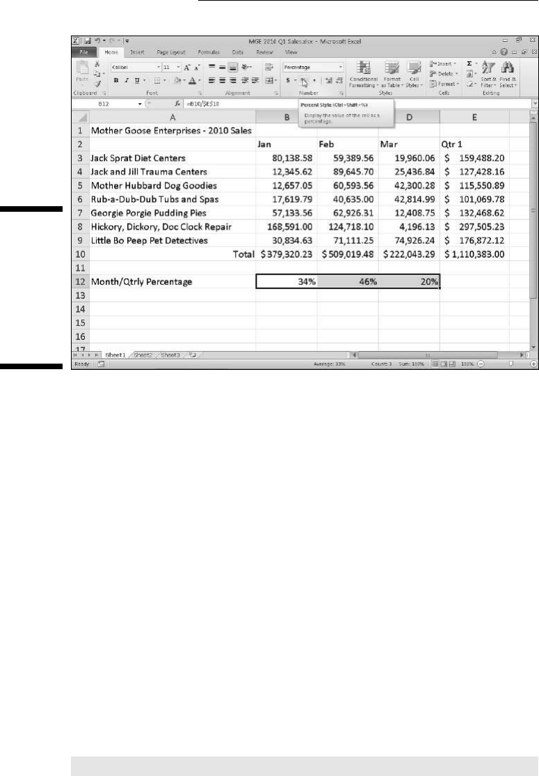
118
Part II: Editing without Tears
Figure 3-14:
Monthly-
to-quarterly
sales
percent-
ages with
Percentage
number
formatting.
Deciding how many decimal places
You can increase or decrease the number of decimal places used in a number
entered by using the Accounting Number Format, Comma Style, or Percent
Style button in the Number group of the Home tab simply by clicking the
Increase Decimal button or the Decrease Decimal button in this group.
Each time you click the Increase Decimal button (the one with the arrow
pointing left), Excel adds another decimal place to the number format you
apply. Percentages appear in the cell range B12:D12 (see Figure 3-15) after
I increase the number of decimal places in the Percent format from none to
two. (Percent Style doesn’t use any decimal places.) I accomplish this by
clicking the Increase Decimal button twice.
The values behind the formatting
Make no mistake about it — all that these fancy number formats do is spiff up
the presentation of the values in the worksheet. Like a good illusionist, a par-
ticular number format sometimes appears to transform some entries, but in
reality, the entries are the same old numbers you started with. For example,
suppose that a formula returns the following value:
25.6456
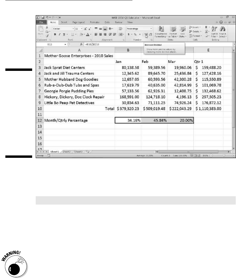
119
Chapter 3: Making It All Look Pretty
Figure 3-15:
Monthly-
to-quarterly
sales per-
centages
after adding
two deci-
mal places
to the
Percentage
number
format.
Now suppose that you format the cell containing this value with the
Accounting Number Format button on the Home tab. The value now appears
as follows:
$25.65
This change may lead you to believe that Excel rounded the value up to two
decimal places. In fact, the program has rounded up only the display of the
calculated value — the cell still contains the same old value of 25.6456. If you
use this cell in another worksheet formula, Excel uses the behind-the-scenes
value in its calculation, not the spiffed-up one shown in the cell.
If you want the values to match their formatted appearance in the worksheet,
Excel can do that in a single step. Be forewarned, however, that this is a one-
way trip. You can convert all underlying values to the way they are displayed
by selecting a single check box, but you can’t return them to their previous
state by deselecting this check box.
Well, because you insist on knowing this little trick anyway, here goes (just
don’t write and try to tell me that you weren’t warned):
1. Make sure that you format all the values in your worksheet with the
right number of decimal places.
You must do this step before you convert the precision of all values in
the worksheet to their displayed form.

120
Part II: Editing without Tears
2. Choose File➪Options➪Advanced or press Alt+FIA to open the
Advanced tab of Excel Options dialog box.
3. In the When Calculating This Workbook section, click the Set
Precision as Displayed check box (to fill it with a check mark).
Excel displays the Data Will Permanently Lose Accuracy alert dialog box.
4. Go ahead (live dangerously) and click the OK button or press Enter to
convert all values to match their display. Click OK again to close the
Excel Options dialog box.
Save the workbook with the calculated values. After converting all the values
in a worksheet by selecting the Set Precision as Displayed check box, open the
Save As dialog box (File➪Save As or press Alt+FA). Edit the filename in the File
Name text box (maybe by appending as Displayed to the current filename)
before you click the Save button or press Enter. That way, you’ll have two
copies: the original workbook file with the values as entered and calculated by
Excel and the new as Displayed version.
Make it a date!
In Chapter 2, I mention that you can easily create formulas that calculate the
differences between the dates and times that you enter in your worksheets.
The only problem is that when Excel subtracts one date from another date
or one time from another time, the program automatically formats the cal-
culated result in a corresponding date or time number format as well. For
example, if you enter 8-15-10 in cell B4 and 4/15/10 in cell C4 and in cell D4
enter the following formula for finding the number of elapsed days between
the two dates:
=B4-C4
Excel correctly returns the result of 122 (days) using the General number
format. However, when dealing with formulas that calculate the difference
between two times in a worksheet, you have to reformat the result that
appears in a corresponding time format into the General format. For example,
suppose that you enter 8:00 AM in cell B5 and 4:00 PM in cell C5 and then
create in cell D5 the following formula for calculating the difference in hours
between the two times:
=C5-B5
You then have to convert the result in cell D5 — that automatically appears as
8:00 AM — to the General format. When you do this, the fraction 0.333333 —

121
Chapter 3: Making It All Look Pretty
representing its fraction of the total 24-hour period — replaces 8:00 AM in cell
D5. You can then convert this fraction of a total day into the corresponding
number of hours by multiplying this cell by 24.
Ogling some of the other number formats
Excel supports more number formats than just the Accounting, Comma
Style, and Percentage number formats. To use them, select the cell range (or
ranges) you want to format and select Format Cells on the cell shortcut menu
(right-click somewhere in the cell selection to activate this menu) or just
press Ctrl+1 to open the Format Cells dialog box.
After the Format Cells dialog box opens with the Number tab displayed,
you select the desired format from the Category list box. Some number
formats — such as Date, Time, Fraction, and Special — give you further for-
matting choices in a Type list box. Other number formats, such as Number
and Currency, have their own particular boxes that give you options for refin-
ing their formats. When you click the different formats in these list boxes,
Excel shows what effect this would have on the first of the values in the cur-
rent cell selection in the Sample area above. When the sample has the format
that you want to apply to the current cell selection, you just click OK or press
Enter to apply the new number format.
Excel contains a nifty category of number formats called Special. The Special
category contains the following four number formats that may interest you:
✓ Zip Code: Retains any leading zeros in the value (important for zip
codes and of absolutely no importance in arithmetic computations).
Example: 00123.
✓ Zip Code + 4: Automatically separates the last four digits from the first
five digits and retains any leading zeros. Example: 00123-5555.
✓ Phone Number: Automatically encloses the first three digits of the
number in parentheses and separates the last four digits from the previ-
ous three with a dash. Example: (999) 555-1111.
✓ Social Security Number: Automatically puts dashes in the value to sepa-
rate its digits into groups of three, two, and four. Example: 666-00-9999.
These Special number formats really come in handy when creating data lists
in Excel that often deal with stuff like zip codes, telephone numbers, and
sometimes even Social Security numbers (see Chapter 9 for more on creating
and using data lists).

122
Part II: Editing without Tears
Calibrating Columns
For those times when Excel 2010 doesn’t automatically adjust the width of
your columns to your complete satisfaction, the program makes your chang-
ing the column widths a breeze. The easiest way to adjust a column is to do
a best-fit, using the AutoFit feature. With this method, Excel automatically
determines how much to widen or narrow the column to fit the longest entry
currently in the column.
Here’s how to use AutoFit to get the best fit for a column:
1. Position the mouse pointer on the right border of the worksheet frame
with the column letter at the top of the worksheet.
The mouse pointer changes to a double-headed arrow pointing left and
right.
2. Double-click the mouse button.
Excel widens or narrows the column width to suit the longest entry.
You can apply a best-fit to more than one column at a time. Simply select all
the columns that need adjusting (if the columns neighbor one another, drag
through their column letters on the frame; if they don’t, hold down the Ctrl
key while you click the individual column letters). After you select the col-
umns, double-click any of the right borders on the frame.
Best-fit à la AutoFit doesn’t always produce the expected results. A long title
that spills into several columns to the right produces a very wide column
when you use best-fit.
When AutoFit’s best-fit won’t do, drag the right border of the column (on the
frame) until it’s the size you need instead of double-clicking it. This manual
technique for calibrating the column width also works when more than one
column is selected. Just be aware that all selected columns assume whatever
size you make the one that you’re actually dragging.
You can also set the widths of columns from the Format button’s drop-down
list in the Cells group on the Home tab. When you click this drop-down
button, the Cell Size section of this drop-down menu contains the following
width options:
✓ Column Width to open the Column Width dialog box where you enter
the number of characters that you want for the column width before you
click OK

123
Chapter 3: Making It All Look Pretty
✓ AutoFit Column Width to have Excel apply best-fit to the columns based
on the widest entries in the current cell selection
✓ Default Width to open the Standard Width dialog box containing the
standard column width of 8.43 characters that you can apply to the col-
umns in the cell selection
Rambling rows
The story with adjusting the heights of rows is pretty much the same as that
with adjusting columns except that you do a lot less row adjusting than you
do column adjusting. That’s because Excel automatically changes the height
of the rows to accommodate changes to their entries, such as selecting a
larger font size or wrapping text in a cell. I discuss both of these techniques
in the upcoming section “Altering the Alignment.” Most row-height adjust-
ments come about when you want to increase the amount of space between a
table title and the table or between a row of column headings and the table of
information without actually adding a blank row. (See the section “From top
to bottom,” later in this chapter, for details.)
To increase the height of a row, drag the bottom border of the row frame
down until the row is high enough and then release the mouse button. To
shorten a row, reverse this process and drag the bottom row-frame border
up. To use AutoFit to best-fit the entries in a row, you double-click the
bottom row-frame border.
As with columns, you can also adjust the height of selected rows using row
options in the Cell Size section on the Format button’s drop-down menu on
the Home tab:
✓ Row Height to open the Row Height dialog box where you enter the
number of points in the Row Height text box and then click OK
✓ AutoFit Row Height to return the height of selected rows to the best fit
Now you see it, now you don’t
A funny thing about narrowing columns and rows: You can get carried away
and make a column so narrow or a row so short that it actually disappears
from the worksheet! This can come in handy for those times when you
don’t want part of the worksheet visible. For example, suppose you have a

124
Part II: Editing without Tears
worksheet that contains a column listing employee salaries — you need these
figures to calculate the departmental budget figures, but you would prefer to
leave sensitive info off most printed reports. Rather than waste time moving
the column of salary figures outside the area to be printed, you can just hide
the column until after you print the report.
Hiding worksheet columns
Although you can hide worksheet columns and rows by just adjusting them
out of existence, Excel does offer an easier method of hiding them, via the
Hide & Unhide option on the Format button’s drop-down menu (located in
the Cells group of the Home tab). Suppose that you need to hide column B
in the worksheet because it contains some irrelevant or sensitive informa-
tion that you don’t want printed. To hide this column, you could follow these
steps:
1. Click anywhere in column B to select the column.
2. Click the drop-down button attached to the Format button in the Cells
group on the Home tab.
Excel opens the Format button’s drop-down menu.
3. Click Hide & Unhide➪Hide Columns on the drop-down menu.
That’s all there is to it — column B goes poof! All the information in the
column disappears from the worksheet. When you hide column B, notice that
the row of column letters in the frame now reads A, C, D, E, F, and so forth.
You could just as well have hidden column B by right-clicking its column letter
on the frame and then choosing the Hide command on the column’s shortcut
menu.
Now, suppose that you’ve printed the worksheet and need to make a change
to one of the entries in column B. To unhide the column, follow these steps:
1. Position the mouse pointer on column letter A in the frame and drag
the pointer right to select both columns A and C.
You must drag from A to C to include hidden column B as part of the
column selection — don’t click while holding down the Ctrl key or you
won’t get B.
2. Click the drop-down button attached to the Format button in the Cells
group on the Home tab.
3. Click Hide & Unhide➪Unhide Columns on the drop-down menu.
Excel brings back the hidden B column, and all three columns (A, B, and C)
are selected. You can then click the mouse pointer on any cell in the work-
sheet to deselect the columns.

125
Chapter 3: Making It All Look Pretty
You could also unhide column B by selecting columns A through C, right-click-
ing either one of them, and then choosing the Unhide command on the column
shortcut menu.
Hiding worksheet rows
The procedure for hiding and unhiding rows of the worksheet is essentially
the same as for hiding and unhiding columns. The only difference is that
after selecting the rows to hide, you click Hide & Unhide➪Hide Rows on the
Format button’s drop-down menu and Hide & Unhide➪Unhide Rows to bring
them back.
Don’t forget that you can use the Hide and Unhide options on the rows’
shortcut menu to make selected rows disappear and then reappear in the
worksheet.
Futzing with the Fonts
When you start a new worksheet, Excel 2010 assigns a uniform font and type
size to all the cell entries you make. The default font varies according to the
version of Windows under which you’re running Excel. When you run Excel
on Windows 7 and Vista, Excel uses its new Calibri font (the so-called Body
Font) in 11-point size, and when running Excel under Windows XP, it uses its
standard Arial font in a 10-point size. Although these two fonts may be fine
for normal entries, you may want to use something with a little more zing for
titles and headings in the worksheet.
If you don’t especially care for the standard font that Excel uses on your
version of Windows, modify it from the General tab of the Excel Options
dialog box (choose File➪Options or press Alt+FI). Look for the Use This Font
drop-down list box (containing Body Font as the default choice) in the When
Creating New Workbooks section and then click the name of new font you
want to make standard from this drop-down list. If you want a different type
size, choose the Font Size drop-down list box and click a new point size on its
drop-down menu or enter the new point size for the standard font directly into
the Font Size text box.
Using the buttons in the Font group on the Home tab, you can make most
font changes (including selecting a new font style or new font size) without
having to resort to changing the settings on the Font tab in the Format Cells
dialog box (Ctrl+1):
✓ To select a new font for a cell selection, click the drop-down button next
to the Font combo box and then select the name of the font you want to
use from the list box. Excel displays the name of each font that appears
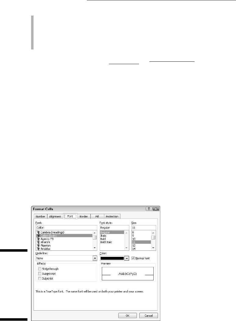
126
Part II: Editing without Tears
in this list box in the actual font named (so that the font name becomes
an example of what the font looks like — onscreen anyway).
✓ To change the font size, click the drop-down button next to the Font Size
combo box, select the new font size or click the Font Size text box, type
the new size, and then press Enter.
You can also add bold, italic, underlining, or strikethrough
to the font you
use. The Font group of the Home tab contains the Bold, Italic, and Underline
buttons, which not only add these attributes to a cell selection but remove
them as well. After you click any of these attribute tools, notice that the
tool becomes shaded whenever you position the cell cursor in the cell or
cells that contain that attribute. When you click a selected format button to
remove an attribute, Excel no longer shades the attribute button when you
select the cell.
Although you’ll probably make most font changes with the Home tab on the
Ribbon, on rare occasions you may find it more convenient to make these
changes from the Font tab in the Format Cells dialog box (Ctrl+1).
As you can see in Figure 3-16, this Font tab in the Format Cells dialog box
brings together under one roof fonts, font styles (bold and italics), effects
(strikethrough, superscript, and subscript), and color changes. When you
want to make many font-related changes to a cell selection, working in the
Font tab may be your best bet. One of the nice things about using this tab is
that it contains a Preview box that shows you how your font changes appear
(onscreen at least).
Figure 3-16:
Use the
Font tab on
the Format
Cells dialog
box to make
many font
changes at
one time.

127
Chapter 3: Making It All Look Pretty
To change the color of the entries in a cell selection, click the Font Color but-
ton’s drop-down menu in the Font group on the Home tab and then select the
color you want the text to appear in the drop-down palette. You can use Live
Preview to see what the entries in the cell selection look like in a particular
font color by moving the mouse pointer over the color swatches in the pal-
ette before you select one by clicking it (assuming, of course, that the palette
doesn’t cover the cells).
If you change font colors and then print the worksheet with a black-and-white
printer, Excel renders the colors as shades of gray. The Automatic option
at the top of the Font Color button’s drop-down menu picks up the color
assigned in Windows as the window text color. This color is black unless you
change it in your display properties. (For help on this subject, please refer to
Microsoft Windows XP For Dummies, Microsoft Windows Vista For Dummies, or
Microsoft Windows 7 For Dummies all by Andy Rathbone — and be sure to tell
Andy that Greg sent ya!)
Altering the Alignment
The horizontal alignment assigned to cell entries when you first make them is
simply a function of the type of entry it is: All text entries are left-aligned, and
all values are right-aligned with the borders of their cells. However, you can
alter this standard arrangement anytime it suits you.
The Alignment group of the Home tab contains three normal horizontal align-
ment tools: the Align Left, Center, and Align Right buttons. These buttons
align the current cell selection exactly as you expect them to. On the right
side of the Alignment group, you usually find the special alignment button
called Merge & Center.
Despite its rather strange name, you’ll want to get to know this button. You
can use it to center a worksheet title across the entire width of a table in sec-
onds (or faster, depending upon your machine). I show you in Figures 3-17
and 3-18 how you can use this tool. In Figure 3-17, notice that the worksheet
title Mother Goose Enterprises – 2010 Sales is in cell A1. To center this title
over the table (which extends from column A through E), select the cell range
A1:E1 (the width of the table) and then click the Merge & Center button in the
Alignment group on the Ribbon’s Home tab.
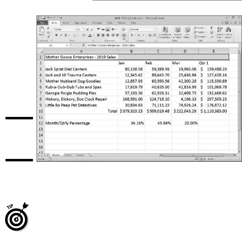
128
Part II: Editing without Tears
Figure 3-17:
A worksheet
title before
merging and
centering.
Look at Figure 3-18 to see the result: The cells in row 1 of columns A through
E are merged into one cell, and now the title is properly centered in this
“super” cell and consequently over the entire table.
If you ever need to split up a supercell that you’ve merged with Merge &
Center back into its original, individual cells, select the cell and then simply
click the Merge & Center button in the Alignment group on the Home tab
again. You can also do this by clicking the drop-down button attached to the
Merge & Center button on the Home tab and then clicking Unmerge Cells on
this drop-down menu (a few more steps, I’d say!).
Intent on indents
In Excel 2010, you can indent the entries in a cell selection by clicking the
Increase Indent button. The Increase Indent button in the Alignment group
of the Home tab sports a picture of an arrow pushing the lines of text to the
right. Each time you click this button, Excel indents the entries in the current
cell selection to the right by three character widths of the standard font. (See
the section “Futzing with the Fonts,” earlier in this chapter, if you don’t know
what a standard font is or how to change it.)
You can remove an indent by clicking the Decrease Indent button (to the
immediate left of the Increase Indent button) on the Home tab with the
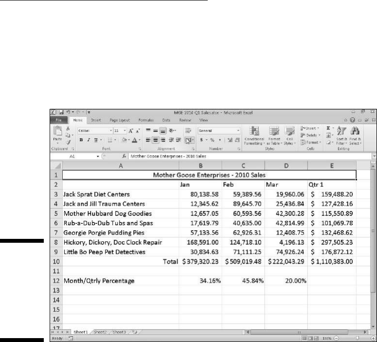
129
Chapter 3: Making It All Look Pretty
picture of the arrow pushing the lines of text to the left. Additionally, you
can change how many characters an entry indents with the Increase Indent
button (or outdents with the Decrease Indent button). Open the Format Cells
dialog box (Ctrl+1). Select the Alignment tab, and then alter the value in the
Indent text box (by typing a new value in this text box or by dialing up a new
value with its spinner buttons).
Figure 3-18:
A worksheet
title after
merging and
centering
it across
columns A
through E.
From top to bottom
Left, right, and center alignment all refer to the horizontal positioning of a text
entry in relation to the left and right cell borders (that is, horizontally). You
can also align entries in relation to the top and bottom borders of their cells
(that is, vertically). Normally, all entries align vertically with the bottom of
the cells (as though they were resting on the very bottom of the cell). You
can also vertically center an entry in its cell or align it with the top of its cell.
To change the vertical alignment of a cell range that you’ve selected, click
the appropriate button (Top Align, Middle Align, or Bottom Align) in the
Alignment group on the Home tab.
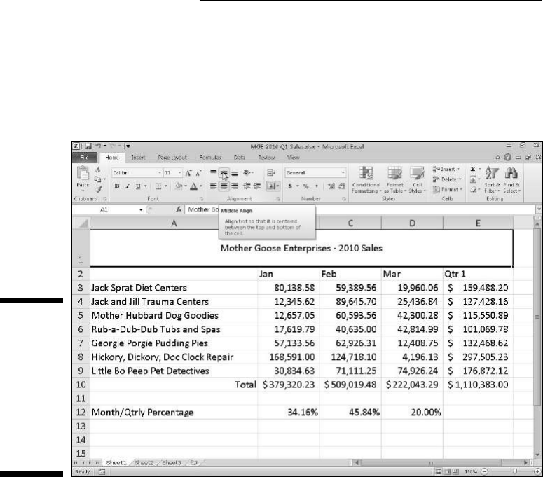
130
Part II: Editing without Tears
Figure 3-19 shows the title for the 2010 Mother Goose Enterprises sales
worksheet after centering it vertically in its cell by clicking the Middle Align
button on the Home tab. (This text entry was previously centered across the
cell range A1:E1; the height of row 1 is increased from the normal 15 points to
36 points.)
Figure 3-19:
The work-
sheet
title after
centering
it vertically
between the
top and bot-
tom edges
of row 1.
Tampering with how the text wraps
Traditionally, column headings in worksheet tables have been a problem —
you had to keep them really short or abbreviate them if you wanted to avoid
widening all the columns more than the data warranted. You can avoid this
problem in Excel by using the Wrap Text button in the Alignment group on
the Home tab (the one to the immediate right of the Orientation button). In
Figure 3-20, I show a new worksheet in which the column headings containing
the various companies within the vast Mother Goose Enterprises conglom-
erate use the Wrap Text feature to avoid widening the columns as much as
these long company names would otherwise require.
To create the effect shown in Figure 3-20, select the cells with the column
headings (the cell range B2:H2) and then click the Wrap Text button in the
Alignment group on the Home tab.
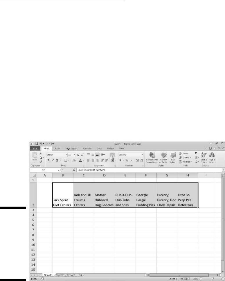
131
Chapter 3: Making It All Look Pretty
Selecting Wrap Text breaks up the long text entries (that either spill over or
cut off) in the selection into separate lines. To accommodate more than one
line in a cell, the program automatically expands the row height so that the
entire wrapped-text entry is visible.
When you select Wrap Text, Excel continues to use the horizontal and
vertical alignment you specify for the cell. You can use any of the Horizontal
alignment options found on the Alignment tab of the Format Cells dialog
box (Ctrl+1), including Left (Indent), Center, Right (Indent), Justify, or
Center Across Selection. However, you can’t use the Fill option or Distrib-
uted (Indent) option. Select the Fill option on the Horizontal drop-down list
box only when you want Excel to repeat the entry across the entire width
of the cell.
If you want to wrap a text entry in its cell and have Excel justify the text
with both the left and right borders of the cell, select the Justify option from
the Horizontal drop-down list box in the Alignment tab in the Format Cells
dialog box.
Figure 3-20:
A new
worksheet
with the
column
headings
formatted
with the
Wrap Text
option.
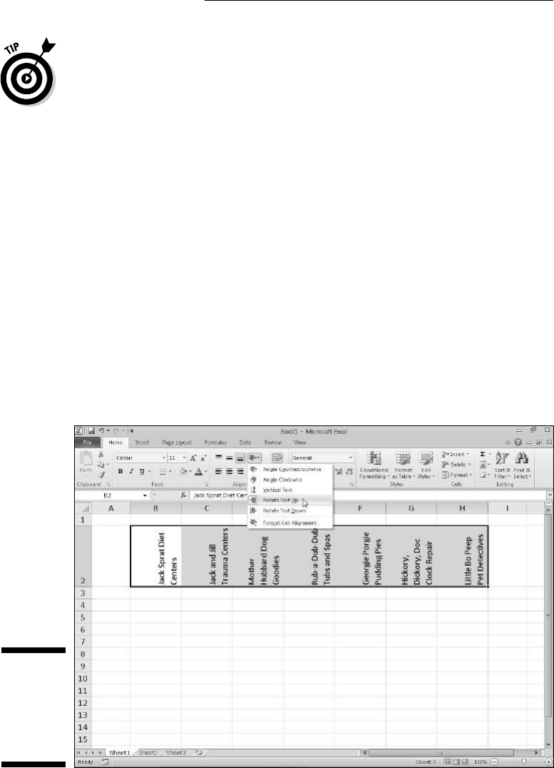
132
Part II: Editing without Tears
You can break a long text entry into separate lines by positioning the insertion
point in the cell entry (or on the Formula bar) at the place where you want the
new line to start and pressing Alt+Enter. Excel expands the row containing the
cell (and the Formula bar above) when it starts a new line. When you press
Enter to complete the entry or edit, Excel automatically wraps the text in the
cell, according to the cell’s column width and the position of the line break.
Reorienting cell entries
Instead of wrapping text entries in cells, you may find it more beneficial to
change the orientation of the text by rotating the text up (in a counterclock-
wise direction) or down (in a clockwise direction). Peruse Figure 3-21 for a
situation where changing the orientation of the wrapped column headings
works much better than just wrapping them in their normal orientation in
the cells.
This example shows the same column headings for the sample order form I
introduced in Figure 3-20 after rotating them 90 degrees counterclockwise. To
make this switch, first select the cell range B2:H2. Next, click the Orientation
button in the Alignment group on the Home tab and then click the Rotate
Text Up option on the drop-down menu.
Figure 3-21:
Column
headings
rotated 90°
counter-
clockwise.
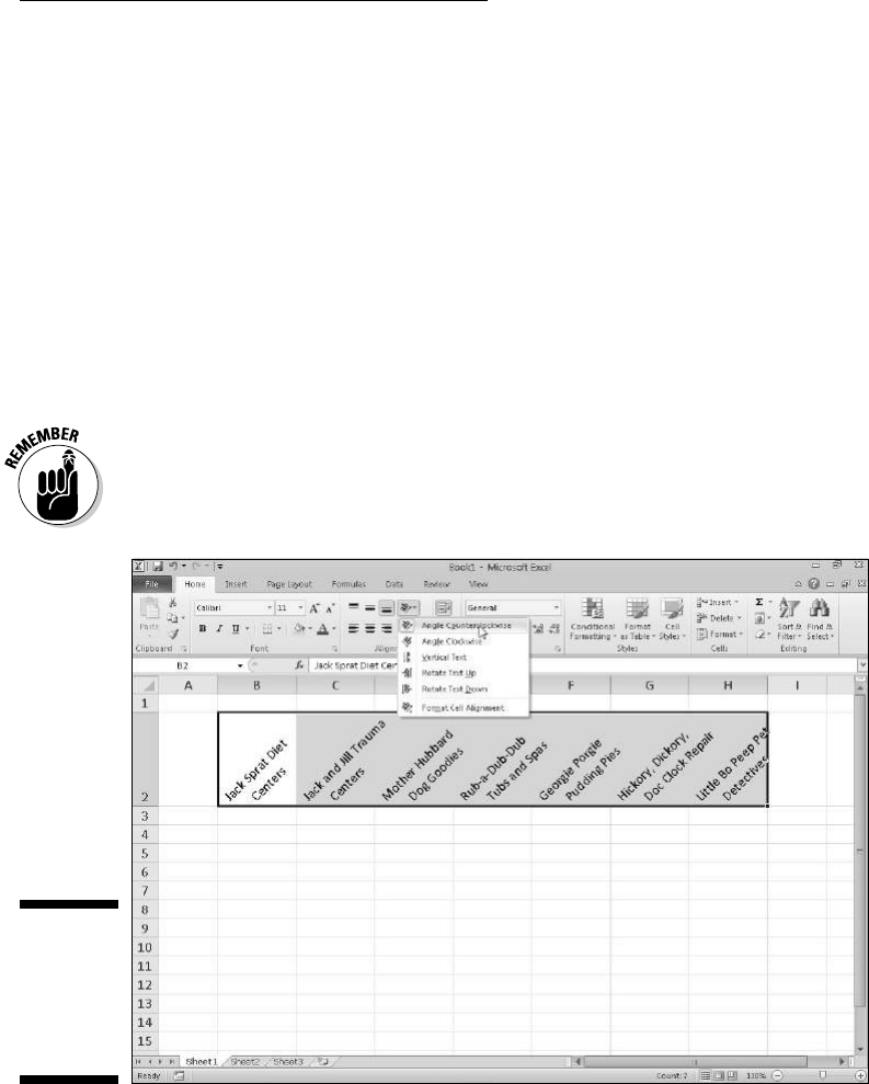
133
Chapter 3: Making It All Look Pretty
Figure 3-22 shows the same headings rotated up at a 45-degree angle. To
create what you see in this figure, you click the Angle Counterclockwise
option on the Orientation button’s drop-down menu after making the same
cell selection, B2:H2.
If you need to set the rotation of the entries in a spreadsheet at angles
other than 45 and 90 degrees (up or down), you need to click the Format
Cell Alignment option on the Orientation button’s drop-down menu. Doing
so opens the Alignment tab of the Format Cells dialog box (or press Ctrl+1
and click the Alignment tab) where you can then use the controls in the
Orientation section to set the angle and number of degrees.
To set a new angle, enter the number of degrees in the Degrees text box, click
the appropriate place on the semicircular diagram, or drag the line extending
from the word Text in the diagram to the desired angle.
To angle text up using the Degrees text box, enter a positive number between
1 and 45 in the text box. To angle the text down, enter a negative number
between –1 and –45.
Figure 3-22:
Column
headings
rotated 45°
counter-
clockwise.

134
Part II: Editing without Tears
To set the text vertically so that each letter is above the other in a single
column, click the Vertical Text option on the Orientation button’s drop-down
menu on the Home tab.
Shrink to fit
For those times when you need to prevent Excel from widening the column
to fit its cell entries (as might be the case when you need to display an entire
table of data on a single screen or printed page), use the Shrink to Fit text
control.
Click the Alignment tab of the Format Cells dialog box (Ctrl+1) and then click
the Shrink to Fit check box in the Text Control section. Excel reduces the font
size of the entries to the selected cells so that they don’t require changing
the current column width. Just be aware when using this Text Control option
that, depending on the length of the entries and width of the column, you can
end up with some text entries so small that they’re completely illegible!
Bring on the borders!
The gridlines you normally see in the worksheet to separate the columns
and rows are just guidelines to help you keep your place as you build your
spreadsheet. You can choose to print them with your data or not (by check-
ing or clearing the Print check box that appears in the Gridlines section of
the Sheet Options group on the Page Layout tab).
To emphasize sections of the worksheet or parts of a particular table, you
can add borderlines or shading to certain cells. Don’t confuse the borderlines
that you add to accent a particular cell selection with the gridlines used to
define cell borders in the worksheet — borders that you add print regardless
of whether you print the worksheet gridlines.
To see the borders that you add to the cells in a worksheet, remove the grid-
lines normally displayed in the worksheet by clearing the View check box in
the Gridlines section of the Sheet Options group on the Page Layout tab.
To add borders to a cell selection, click the drop-down button attached to
the Borders button in the Font group on the Home tab. This displays a drop-
down menu with all the border options you can apply to the cell selection
(see Figure 3-23) where you click the type of line you want to apply to all
its cells.
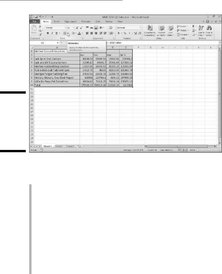
135
Chapter 3: Making It All Look Pretty
Figure 3-23:
Select
borders for
a cell selec-
tion with the
Borders but-
ton on the
Home tab.
When selecting options on this drop-down menu to determine where you
want the borderlines drawn, keep these things in mind:
✓ To have Excel draw borders only around the outside edges of the entire
cell selection (in other words, following the path of the expanded cell
cursor), click the Outside Borders or the Thick Box Border options on
this menu. To draw the outside borders yourself around an unselected
cell range in the active worksheet, click the Draw Border option, drag
the mouse (using the Pencil mouse pointer) through the range of cells,
and then click the Borders button on the Home tab’s Font group.
✓ If you want borderlines to appear around all four edges of each cell in
the cell selection (like a paned window), select the All Borders option
on this drop-down menu. If you want to draw the inside and outside bor-
ders yourself around an unselected cell range in the active worksheet,
click the Draw Border Grid option, drag the mouse (using the Pencil
mouse pointer) through the range of cells, and then click the Borders
button on the Home tab.
To change the type of line, line thickness, or color of the borders you apply
to a cell selection, you must open the Format Cells dialog box and use the
options on its Border tab (click More Borders at the bottom of the Borders
button’s drop-down menu or press Ctrl+1 and then click the Border tab).

136
Part II: Editing without Tears
To select a new line thickness or line style for a border you’re applying, click
its example in the Style section. To change the color of the border you want
to apply, click the color sample on the Color drop-down palette. After you
select a new line style and/or color, apply the border to the cell selection by
clicking the appropriate line in either the Presets or Border section of the
Border tab before you click OK.
To get rid of existing borders in a worksheet, you must select the cell or cells
that presently contain them and then click the No Border option at the top of
the second section on the Borders button’s drop-down menu.
Applying fill colors, patterns,
and gradient effects to cells
You can also add emphasis to particular sections of the worksheet or one of
its tables by changing the fill color of the cell selection and/or applying a pat-
tern or gradient to it.
If you’re using a black-and-white printer, you want to restrict your color
choices to light gray in the color palette. Additionally, you want to restrict
your use of pattern styles to the very open ones with few dots when enhanc-
ing a cell selection that contains any kind of entries (otherwise, the entries will
be almost impossible to read when printed).
To choose a new fill color for the background of a cell selection, you can
click the Fill Color button’s drop-down menu in the Font group on the Home
tab and then select the color you want to use in the drop-down palette.
Remember that you can use Live Preview to see what the cell selection looks
like in a particular fill color by moving the mouse pointer over the color
swatches. Click one to select it.
To choose a new pattern for a cell selection, you must open the Format Cells
dialog box (Ctrl+1), and then click the Fill tab. To change the pattern of the
cell selection, click a pattern swatch from the Pattern Style button’s pattern
palette. To add a fill color to the pattern you select, click its color swatch in
the Background Color section of the Fill tab.
If you want to add a gradient effect to the cell selection that goes from one
color to another in a certain direction, click the Fill Effects button on the
Fill tab to open the Fill Effects dialog box (see Figure 3-24). This dialog box
contains a Gradient tab with controls that enable you to determine the two
colors to use as well as shading style and variant.
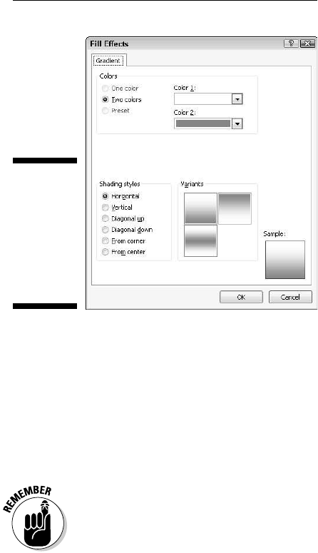
137
Chapter 3: Making It All Look Pretty
Figure 3-24:
Select a
new gradi-
ent for a cell
selection
in the Fill
Effects
dialog box.
After you select the colors and styles of the gradient, check the Sample
swatch in the Fill Effects dialog box. When you have it the way you want it,
click OK to close the Fill Effects dialog box and return to the Format Cells
dialog box. The selected gradient effect then appears in its Sample area on
the Fill tab in the Format Cells dialog box. Unfortunately, this is one area
where Live Preview doesn’t work, so you’re just going to have to click its OK
button to apply the gradient to the cell selection to see how it actually looks
in the worksheet.
Although you can’t select new patterns or gradients (only colors) with the Fill
Color button on the Home tab, you can remove fill colors, patterns, and gradi-
ents assigned to a cell selection by clicking the No Fill option on the Fill Color
button’s drop-down menu.
Do It in Styles
In Excel 2010, cell styles really come alive in the form of the new Cell Styles
gallery that you open by clicking the Cell Styles button in the Styles group on
the Home tab. The Cell Styles gallery contains loads of readymade styles you
can immediately apply to the current cell selection. Simply click the desired
style sample in the gallery after using the Live Preview feature to determine
which style looks best on your data.

138
Part II: Editing without Tears
Creating a new style for the gallery
To create a new style for the gallery by example, manually format a single
cell with all the attributes you want (font, font size, font color, bold, italic,
underlining, fill color, pattern, borders, orientation, and so on) and then click
the Cell Styles button on the Home tab followed by the New Cell Style option
at the bottom of the gallery. Excel then opens a Style dialog box where you
replace the generic style name (Style 1, Style 2, and so on) with your own
descriptive name before you click OK.
Excel then adds a sample of your new style — the style name formatted, with
the new style’s attributes — to a Custom section at the top of the Cell Styles
gallery. To apply this custom style to a cell selection, you then only have to
click its sample in the Custom section of the Cell Styles gallery.
The custom cell styles you create don’t become part of the current workbook
until the next time you save the workbook. Therefore, you need to remember
to click the Save button on the Quick Access toolbar or press Ctrl+S to save
your changes after creating a new cell style if you want that style to remain
part of the workbook’s Cell Styles gallery the next time you open the work-
book in Excel.
Copying custom styles from
one workbook into another
Excel makes it easy to copy custom cell styles that you’ve saved as part
of one workbook into the workbook you’re currently working on. To copy
custom styles from one workbook to another, follow these steps:
1. Open the workbook that needs the custom styles added to it from
another existing workbook.
This can be a brand new workbook or one that you’ve opened for editing
(see Chapter 4).
2. Open the workbook that has the custom styles you want to copy saved
as part of it.
See the previous section, “Creating a new style for the gallery” for tips
on how to create and save cell styles.
3. Switch back to the workbook into which you want to copy the saved
custom styles.
You can do this by clicking the workbook’s button on the Windows
taskbar or using the Flip feature by pressing Alt+Tab until you select the
workbook’s thumbnail in the center of the display.

139
Chapter 3: Making It All Look Pretty
4. Click the Cell Styles button on the Home tab followed by Merge Styles
in the Cell Styles gallery or press Alt+HJM.
Excel opens the Merge Styles dialog box.
5. Click the name of the open workbook file that contains the custom
styles to copy in the Merge Styles From list box and then click OK.
After you close the Merge Styles dialog box, Excel adds all the custom styles
from the designated workbook into the current workbook adding it to the
Custom section of its Cell Styles gallery. To retain the custom styles you
just imported, save the current workbook (Save button on the Quick Access
toolbar or Ctrl+S). Then, you can switch back to the workbook containing the
original custom styles you just copied and close its file (Alt+FC).
Fooling Around with the Format Painter
Using cell styles to format ranges of worksheet cells is certainly the way to
go when you have to apply the same formatting repeatedly in the workbooks
you create. However, there may be times when you simply want to reuse
a particular cell format and apply it to particular groups of cells in a single
workbook without ever bothering to open the Cell Styles gallery.
For those occasions when you feel the urge to format on the fly (so to speak),
use the Format Painter button (the paintbrush icon) in the Clipboard group
on the Home tab. This wonderful little tool enables you to take the formatting
from a particular cell that you fancy up and apply its formatting to other cells
in the worksheet simply by selecting those cells.
To use the Format Painter to copy a cell’s formatting to other worksheet
cells, just follow these easy steps:
1. Format an example cell or cell range in your workbook, selecting
whatever fonts, alignment, borders, patterns, and color you want it to
have.
2. With the cell cursor in one of the cells you just fancied up, click the
Format Painter button in the Clipboard group on the Home tab.
The mouse pointer changes from the standard thick, white cross to a
thick, white cross with an animated paintbrush by its side, and you see a
marquee around the selected cell with the formatting to be used by the
Format Painter.
3. Drag the white-cross-plus-animated-paintbrush pointer (the Format
Painter pointer) through all the cells you want to format.
As soon as you release the mouse button, Excel applies all the format-
ting used in the example cell to all the cells you just selected!

140
Part II: Editing without Tears
To keep the Format Painter selected so that you can format a bunch of dif-
ferent cell ranges with the Format Painter pointer, double-click the Format
Painter button on the Home tab after you select the sample cell with the
desired formatting. To stop formatting cells with the Format Painter pointer,
you simply click the Format Painter button on the Home tab again (it remains
selected when you double-click it) to restore the button to its unselected
state and return the mouse pointer to its normal thick, white cross shape.
You can use the Format Painter to restore a cell range that you gussied all up
back to its boring default (General) cell format. To do this, click an empty, pre-
viously unformatted cell in the worksheet before you click the Format Painter
button and then use the Format Painter pointer to drag through the cells you
want returned to the default General format.
Conditional Formatting
Before leaving behind the scintillating subject of cell formatting, there’s one
more formatting button in the Styles group of the Home tab of which you
need to be aware. The Conditional Formatting button enables you to apply
provisional formatting to a cell range based solely on the categories into
which its current values fall. The cool thing about this kind of conditional
formatting is that should you edit the numbers in the cell range so that their
values fall into other categories, the program automatically changes their cell
formatting to suit.
When you click the Conditional Formatting button in the Styles group of the
Home tab, a drop-down menu appears with the following options:
✓ Highlight Cells Rules opens a continuation menu with various options
for defining formatting rules that highlight the cells in the cell selection
that contain certain values, text, or dates; that have values greater or
less than a particular value; or that fall within a certain ranges of values.
✓ Top/Bottom Rules opens a continuation menu with various options for
defining formatting rules that highlight the top and bottom values, per-
centages, and above and below average values in the cell selection.
✓ Data Bars opens a palette with different color data bars that you can
apply to the cell selection to indicate their values relative to each other
by clicking the data bar thumbnail.
✓ Color Scales opens a palette with different two- and three-colored scales
that you can apply to the cell selection to indicate their values relative
to each other by clicking the color scale thumbnail.

141
Chapter 3: Making It All Look Pretty
✓ Icon Sets opens a palette with different sets of icons that you can apply
to the cell selection to indicate their values relative to each other by
clicking the icon set.
✓ New Rule opens the New Formatting Rule dialog box where you define a
custom conditional formatting rule to apply to the cell selection.
✓ Clear Rules opens a continuation menu where you can remove condi-
tional formatting rules for the cell selection by clicking the Clear Rules
from Selected Cells option, for the entire worksheet by clicking the Clear
Rules from Entire Sheet option, or for just the current data table by
clicking the Clear Rules from This Table option.
✓ Manage Rules opens the Conditional Formatting Rules Manager dialog
box where you edit and delete particular rules as well as adjust their
rule precedence by moving them up or down in the Rules list box.
Conditionally formatting values with sets
of graphic scales and markers
The easiest conditional formatting that you can apply to a worksheet cell
range is using the pop-up palettes of graphical scales and markers attached
to the Data Bars, Color Scales, and Icon Sets options on the Conditional
Formatting button’s drop-down menu:
✓ Data Bars represents the relative values in the cell selection by the
length of the color bar in each cell and are great for helping you quickly
spot the lower and higher values within a large range of data.
✓ Color Scales classify the relative values in a cell selection with a color
gradation using a one-, two-, or three-color scale and are great for identi-
fying the distribution of values across a large range of data.
✓ Icon Sets classify the values in the cell selection into three to five cat-
egories and each icon within the set represents a range of values that go
from high to low. Icon sets are great for quickly identifying the different
ranges of values in a range of data.
Figure 3-25 shows you an example of cell ranges (containing identical values)
using each of the three formatting types. The values in the first range
(B2:B12) are conditionally formatted using blue Gradient Fill Data Bars. The
values in the second range (D2:D12) are conditionally formatted using the
Green, Yellow, Red Color Scale. The values in the third range (F2:F12) are
conditionally formatted using the 3 Arrows Directional Icon set.
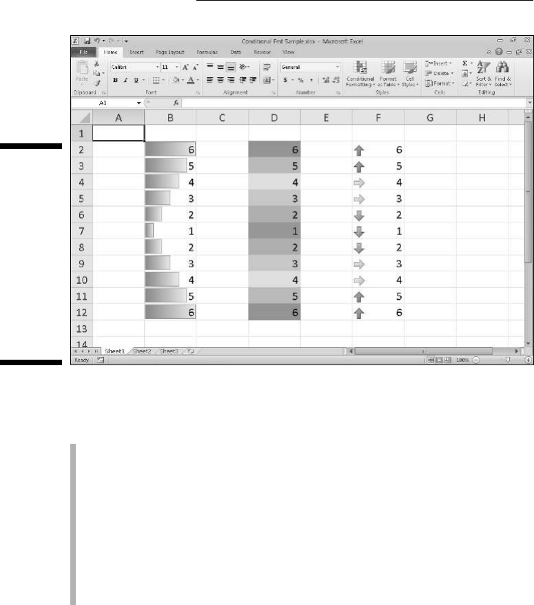
142
Part II: Editing without Tears
Figure 3-25:
Sample
worksheet
with three
identical
cell ranges
format-
ted with
Excel’s Data
Bars, Color
Scales, and
Icon Sets
options.
In Figure 3-25, the particular conditional formatting types Excel assigned to
each cell range can be interpreted as follows:
✓ Data bars added to the cells in the first cell range, B2:B12, represent the
relative size of its values graphically, much like a standard bar chart.
✓ Color scale applied to the second range, D2:D12, represent the relative
size of the values in the range by color and hue (red hues applied to
the lower values, yellow to the middle values, and green to the higher
values).
✓ Directional icons applied to the third cell range, F2:F12, represent the
relative size of the values in the range with arrow icons pointing in dif-
ferent directions (arrows pointing straight down for the lower values,
straight up for the higher values, and sideways for middling values).
Highlighting cells according to what
ranges the values fall into
The Highlight Cells Rules and Top/Bottom Rules options on Excel’s
Conditional Formatting drop-down menu enable you to quickly identify cell
entries of particular interest in various cell ranges in your worksheet.

143
Chapter 3: Making It All Look Pretty
The options on the Highlight Cells Rules continuation menu enable you to set
formats that identify values that are greater than, less than, equal to, or even
between particular values that you set. This menu also contains an option for
setting special formats for identifying cells that contain particular text (such
as Yes, No, or even Maybe answers in a data list) or certain dates (such as
project milestones and deadlines).
Perhaps one of the most useful options on the Highlight Cells Rules continu-
ation menu is the Duplicate Values option that enables you to flag duplicate
entries in a cell range by assigning them a special formatting. Doing this not
only makes it easy to visually identify duplicate entries in a data list or table
but also to find them electronically by searching for their particular formatting
characteristics. (See Chapter 6 for details on searching your worksheets.)
The options on the Top/Bottom Rules continuation menu enable you to spe-
cially format and, therefore, easily identify values in data tables and lists that
are either above or below the norm. These options not only include those
for automatically formatting all values in a range that are among the top 10
highest or lowest (either in value or percentage) but also above or below the
average (as calculated by dividing the total by the number of values).
In addition to using the ready-made rules for conditional formatting located on
the Highlight Cells Rules and Top/Bottom Rules continuation menus, you can
also create your own custom rules. When you create a custom rule, you not
only specify the rule type that identifies which values or text entries to format,
but also you format the colors and other aspects included in the formatting.
(For details on creating custom conditional formats, consult my Excel 2010 All-
in-One For Dummies.)

144
Part II: Editing without Tears

Chapter 4
Going Through Changes
In This Chapter
▶ Opening workbook files for editing
▶ Undoing your boo-boos
▶ Moving and copying with drag and drop
▶ Copying formulas
▶ Moving and copying with Cut, Copy, and Paste
▶ Deleting cell entries
▶ Deleting and inserting columns and rows
▶ Spell-checking the worksheet
▶ Corroborating cell entries with the Text to Speech feature
P
icture this: You just finished creating, formatting, and printing a major
project with Excel — a workbook with your department’s budget for
the next fiscal year. Because you finally understand a little bit about how the
Excel thing works, you finish the job in crack time. You’re actually ahead of
schedule.
You turn the workbook over to your boss so that she can check the num-
bers. With plenty of time for making those inevitable last-minute corrections,
you’re feeling on top of this situation.
Then comes the reality check — your boss brings the document back, and
she’s plainly agitated. “We forgot to include the estimates for the temps and
our overtime hours. They go right here. While you’re adding them, can you
move these rows of figures up and those columns over?”
As she continues to suggest improvements, your heart begins to sink. These
modifications are in a different league than, “Let’s change these column head-
ings from bold to italic and add shading to that row of totals.” Clearly, you’re
looking at a lot more work on this baby than you had contemplated. Even
worse, you’re looking at making structural changes that threaten to unravel
the very fabric of your beautiful worksheet.

146
Part II: Editing without Tears
As the preceding fable points out, editing a worksheet in a workbook can
occur on different levels:
✓ You can make changes that affect the contents of the cells, such as
copying a row of column headings or moving a table to a new area in a
particular worksheet.
✓ You can make changes that affect the structure of a worksheet itself,
such as inserting new columns or rows (so that you can enter new data
originally left out) or deleting unnecessary columns or rows from an
existing table so that you don’t leave any gaps.
✓ You can even make changes to the number of worksheets in a workbook
(by either adding or deleting sheets).
In this chapter, you discover how to make these types of changes safely to a
workbook. As you see, the mechanics of copying and moving data or insert-
ing and deleting rows are simple to master. It’s the impact that such actions
have on the worksheet that takes a little more effort to understand. Not to
worry! You always have the Undo feature to fall back on for those (hopefully
rare) times when you make a little tiny change that throws an entire work-
sheet into complete and utter chaos.
In the final section of this chapter (“Stamping Out Errors with Text to
Speech”), find out how to use the Text to Speech feature to check out and
confirm the accuracy of the data entries you make in your worksheets.
With Text to Speech, you can listen to your computer read back a series of
cell entries while you visually corroborate their accuracy from the original
source document. Text to Speech can make this sort of routine and otherwise
labor-intensive editing much easier and greatly increase the accuracy of your
spreadsheets.
Opening the Darned Thing Up for Editing
Before you can do any damage — I mean, make any changes — in a work-
book, you have to open it up in Excel. To open a workbook, you can choose
File➪Open, press Alt+FO, or use the old standby keyboard shortcuts Ctrl+O
or Ctrl+F12.
Operating the Open dialog box
If you’re running Excel 2010 under Windows 7, an Open dialog box very much
like the one in Figure 4-1 appears. This dialog box is divided into panes: the
Navigation pane on the left where you can select a new folder to open and
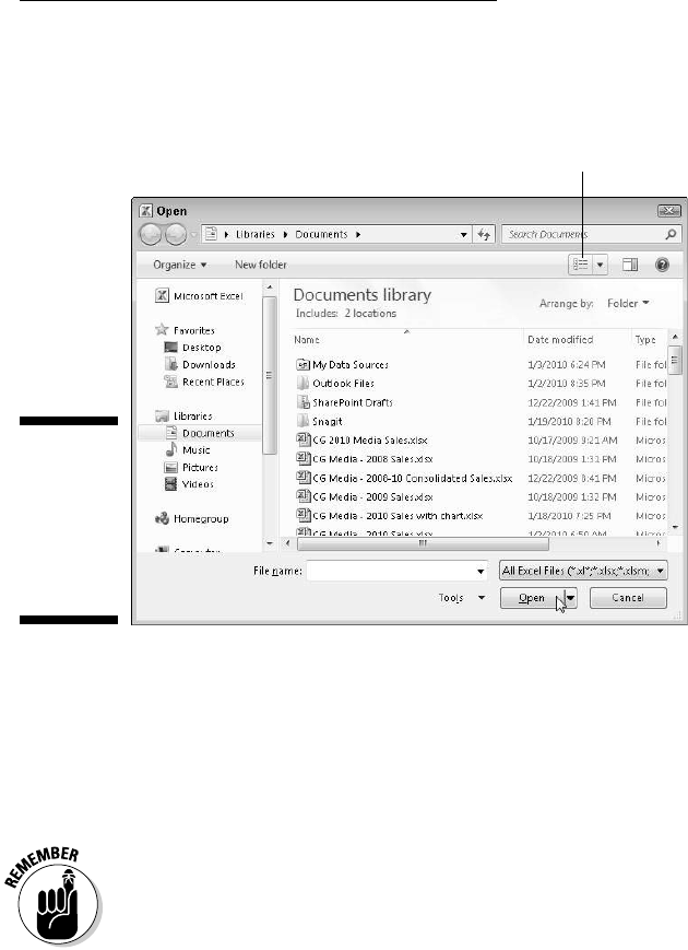
147
Chapter 4: Going Through Changes
the main pane on the right showing the icons for all the subfolders in the cur-
rent folder as well as the documents that Excel can open.
Figure 4-1:
Use the
Open dialog
box to find
and open a
workbook
for editing.
Change your view
The folder with contents displayed in the Open dialog box is either the one
designated as the Default File Location on the Save tab of the Excel Options
dialog box or the folder you last opened during your current Excel work ses-
sion. If you haven’t changed the default folder location since installing Excel
2010 on your computer, this default folder is the Documents Library (simply
referred to as Documents in Windows Vista).
If you’re running Excel 2010 on Windows Vista, your Open dialog box is similar
to the one shown in Figure 4-1 except that your Navigation pane contains a
Folders item instead of Libraries under your list of Favorites. Additionally, the
Views button appears between the Organize and New Folder buttons and not
to their right above the Navigation and main panes.
To open a workbook in another folder, click its link in the Favorite Links sec-
tion of the Navigation pane or click the Expand Folders button (the one with
the triangle pointing upward) and click its folder in this list.
If you open a new folder and it appears empty of all files (and you know that
it’s not an empty folder), this just means the folder doesn’t contain any of
the types of files that Excel can open directly (such as workbooks, template

148
Part II: Editing without Tears
files, and macro sheets). To display all the files whether or not Excel can
open them directly (meaning without some sort of conversion), click the
drop-down button that appears next to the drop-down list box that currently
displays All Excel Files and then click All Files on its drop-down menu.
When the icon for the workbook file you want to work with appears in the
Open dialog box, you can then open it either by clicking its file icon and then
clicking the Open button or, if you’re handy with the mouse, by just double-
clicking the file icon.
You can use the slider attached to the Views drop-down list button in the
Open dialog box to change the way folder and file icons appear in the dialog
box. When you select Large Icons or Extra Large Icons on this slider (or any-
where in between), the Excel workbook icons actually show a preview of the
data in the upper-left corner of the first worksheet when the file is saved with
the preview picture option turned on:
✓ To enable the preview feature when saving workbooks in Excel 2010,
select the Save Thumbnail check box in the Save As dialog box before
saving the file for the first time.
✓ To enable the preview feature when saving workbooks in Excel 97
through 2003, click the Save Preview Picture check box on the Summary
tab of the workbook’s Properties dialog box (File➪Properties) before
saving the file for the first time.
This preview of part of the first sheet can help you quickly identify the work-
book you want to open for editing or printing.
Opening more than one
workbook at a time
If you know that you’re going to edit more than one of the workbook files
shown in the list box of the Open dialog box, you can select multiple files in
the list box and Excel will then open all of them (in the order they’re listed)
when you click the Open button or press Enter.
Remember that in order to select multiple files that appear sequentially in the
Open dialog box, you click the first filename and then hold down the Shift key
while you click the last filename. To select files that aren’t listed sequentially,
you need to hold down the Ctrl key while you click the various filenames.
After the workbook files are open in Excel, you can then switch documents
by selecting their filename buttons on the Windows taskbar or by using the
Flip feature (Alt+Tab) to select the workbook’s thumbnail. (See Chapter 7 for
detailed information on working on more than one worksheet at a time.)

149
Chapter 4: Going Through Changes
Opening recently edited workbooks
If you know that the workbook you now need to edit is one of those that you
opened recently, you don’t even have to fool around with the Open dialog
box. Just choose File➪Recent to display a Recent Workbooks list to the right
of the pull-down menu (or press Alt+FR) and then click the name of the work-
book to open for editing.
When you open the Recent Workbooks list by pressing Alt+FR, Excel displays
the number hot keys to each of the recently opened spreadsheet files in
the list and you then can open the one you need to edit simply by typing its
number.
Excel 2010 automatically keeps a running list of the last 20 files you opened
in the Recent Workbooks list on the File tab. If you want, you can have Excel
display more or fewer files in this list on the File tab.
To change the number of recently opened files that appear, follow these
simple steps:
1. Choose File➪Options➪Advanced or press Alt+FIA to open the
Advanced tab of the Excel Options dialog box.
2. Type a new entry (between 1 and 50) in the Show This Number of
Recent Documents text box or use the spinner buttons to increase or
decrease this number.
3. Click OK or press Enter to close the Excel Options dialog box.
The Open dialog box in Excel 2010
running on Windows XP
The Open dialog box for Windows XP is
arranged a bit differently from the one in
Windows 7 and Windows Vista. This Open
dialog box is divided into two sections: a My
Places panel on the left and a folder and file list
box on the right. If the folder open in the list box
is not the one that has the workbook file you
need to use, use the Up One Level button in the
Open dialog box to change levels until you see
the folder you want to open. Use the buttons
displayed in the My Places panel on the left side
of the Open dialog box (My Recent Documents,
Desktop, My Documents, My Computer, and My
Network Places) to open any folders associated
with these buttons that contain workbook files.
When you locate the file that you want to use
in the list box in the Open dialog box, open it by
clicking its file icon and then clicking the Open
button or pressing Enter (or by double-clicking
the file icon).
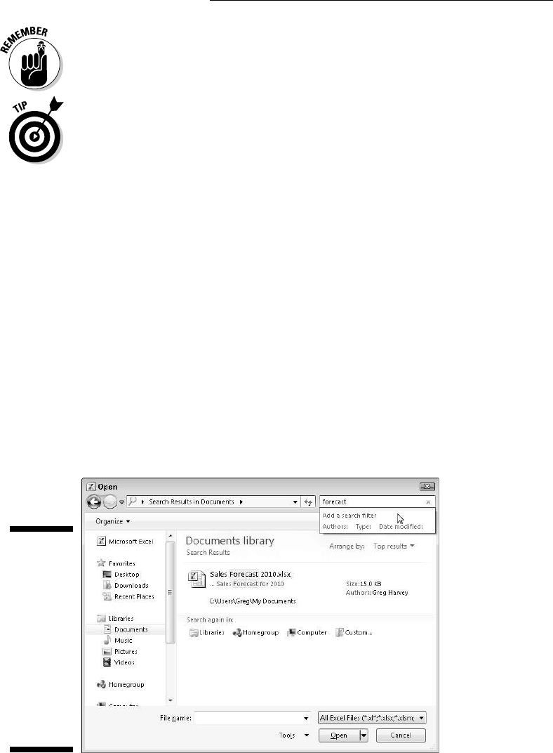
150
Part II: Editing without Tears
If you don’t want any files displayed in the Recent Workbooks list on the File
tab, enter 0 in the Show This Number of Recent Documents text box or select
it with the spinner buttons.
Select the Quickly Access This Number of Recent Workbooks check box on
the Recent Workbooks panel in the Backstage View to have Excel display the
four most recently opened workbooks as items on the File tab. That way, you
can open any of them by clicking its button without having to open the Recent
Workbooks panel. After selecting the Quickly Access This Number of Recent
Workbooks check box, you change the number of recently opened workbooks
added to the File tab by entering the new number in its text box or selecting
the number with its spinner buttons.
When you don’t know where to find them
The only problem you can encounter in opening a document from the Open
dialog box is locating the filename. Everything’s hunky-dory as long as you
can see the workbook filename listed in the Open dialog box or know which
folder to open in order to display it. But what about those times when a file
seems to migrate mysteriously and can’t be found on your computer?
When you run Excel 2010 under Windows 7 or Vista, the operating system
adds a Search Documents text box (simply called Search in Vista) to the
Open dialog box (see Figure 4-2). You can use this text box to search for
missing workbooks from within the Open dialog box.
Figure 4-2:
Use the
Search
Documents
text box in
the Open
dialog box
to quickly
search for
any Excel
workbook
on your
computer.

151
Chapter 4: Going Through Changes
To find a missing workbook, click this search text box in the upper-right
corner of the Open dialog box and then begin typing characters used in the
workbook’s filename or contained in the workbook itself.
As Windows finds any matches for the characters you type, the names of the
workbook files (and other Excel files such as templates and macro sheets as
well) appear in the Open dialog box. As soon as the workbook you want to
open is listed, you can open it by clicking its icon and filename followed by
the Open button or by double-clicking it.
The Open dialog box in Excel 2010 when running under Windows XP does not
have a search feature built in to it. This means that to search for missing work-
books, you have to do it outside Excel by using Windows XP’s search feature
available on its Start menu.
Opening files with a twist
The drop-down button attached to the Open command button at the bottom
of the Open dialog box enables you to open the selected workbook file(s) in a
special way, including:
✓ Open Read-Only: This command opens the files you select in the Open
dialog box’s list box in a read-only state, which means that you can look
but you can’t touch. (Actually, you can touch; you just can’t save your
changes.) To save changes in a read-only file, you must use the Save As
command (File➪Save As or Alt+FA) and give the workbook file a new file-
name. (Refer to Chapter 2.)
✓ Open as Copy: This command opens a copy of the files you select in the
Open dialog box. Use this method of opening files as a safety net: If you
mess up the copies, you always have the originals to fall back on.
✓ Open in Browser: This command opens workbook files you save as Web
pages (which I describe in Chapter 12) in your favorite Web browser.
This command isn’t available unless the program identifies that the
selected file or files were saved as Web pages rather than plain old Excel
workbook files.
✓ Open in Protected View: This command opens the workbook file in
Protected View mode that keeps you from making any changes to the
contents of its worksheets until you click the Enable Editing button that
appears in the orange Protected View panel at the top of the screen.
✓ Open and Repair: This command attempts to repair corrupted work-
book files before opening them in Excel. When you select this command,
a dialog box appears giving you a choice between attempting to repair

152
Part II: Editing without Tears
the corrupted file or opening the recovered version, extracting data
from the corrupted file, and placing it in a new workbook (which you
can save with the Save command). Click the Repair button to attempt
to recover and open the file. Click the Extract Data button if you tried
unsuccessfully to have Excel repair the file.
Much Ado about Undo
Before you start tearing into the workbook that you just opened, get to know
the Undo feature, including how it can put right many of the things that
you could inadvertently mess up. The Undo command button on the Quick
Access toolbar is a regular chameleon button. When you delete the cell selec-
tion by pressing the Delete key, the Undo button’s ScreenTip reads Undo
Clear (Ctrl+Z). If you move some entries to a new part of the worksheet by
dragging it, the Undo command button ScreenTip changes to Undo Drag and
Drop (Ctrl+Z).
In addition to clicking the Undo command button (in whatever guise it
appears), you can also choose this command by pressing Ctrl+Z (perhaps for
unZap).
The Undo command button on the Quick Access toolbar changes in response
to whatever action you just took; that is, it changes after each action. If you
forget to strike when the iron is hot, so to speak, and don’t use the Undo feature
to restore the worksheet to its previous state before you choose another com-
mand, you then need to consult the drop-down menu on the Undo button. Click
its drop-down button that appears to the right of the Undo icon (the curved
arrow pointing to the left). After the Undo drop-down menu appears, click the
action on this menu that you want undone. Excel will then undo this action and
all actions that precede it in the list (which are selected automatically).
Undo is Redo the second time around
After using the Undo command button on the Quick Access toolbar, Excel
2010 activates the Redo command button to its immediate right. If you delete
an entry from a cell by pressing the Delete key and then click the Undo com-
mand button or press Ctrl+Z, the ScreenTip that appears when you position
the mouse pointer over the Redo command button reads Redo Clear (Ctrl+Y).
When you click the Redo command button or press Ctrl+Y, Excel redoes the
thing you just undid. Actually, this sounds more complicated than it is. It
simply means that you use Undo to switch between the result of an action
and the state of the worksheet just before that action until you decide how
you want the worksheet (or until the cleaning crew turns off the lights and
locks up the building).

153
Chapter 4: Going Through Changes
What ya gonna do when you can’t Undo?
Just when you think it is safe to begin gutting the company’s most important
workbook, I really feel that I have to tell you that (yikes!) Undo doesn’t work
all the time! Although you can undo your latest erroneous cell deletion, bad
move, or unwise copy, you can’t undo your latest rash save. (You know, like
when you meant to choose Save As from the File tab to save the edited work-
sheet under a different document name but chose Save and ended up saving
the changes as part of the current document.)
Unfortunately, Excel doesn’t let you know when you are about to take a step
from which there is no return — until it’s too late. After you’ve gone and
done the un-undoable and you click the Undo button where you expect its
ScreenTip to say Undo blah, blah, it now reads Can’t Undo.
One exception to this rule is when the program gives you advance warning
(which you should heed). When you choose a command that is normally pos-
sible but because you’re low on memory or the change will affect so much
of the worksheet, or both, Excel knows that it can’t undo the change if it
goes through with it, the program displays an alert box telling you that there
isn’t enough memory to undo this action and asking whether you want to go
ahead anyway. If you click the Yes button and complete the edit, just realize
that you do so without any possibility of pardon. If you find out, too late, that
you deleted a row of essential formulas (that you forgot about because you
couldn’t see them), you can’t bring them back with Undo. In such a case, you
would have to close the file (File➪Close) and NOT save your changes.
Doing the Old Drag-and-Drop Thing
The first editing technique you need to learn is drag and drop. As the name
implies, you can use this mouse technique to pick up a cell selection and
drop it into a new place on the worksheet. Although drag and drop is primar-
ily a technique for moving cell entries around a worksheet, you can adapt it
to copy a cell selection, as well.
To use drag and drop to move a range of cell entries (one cell range at a
time), follow these steps:
1. Select a cell range.
2. Position the mouse pointer on one edge of the extended cell cursor
that now surrounds the entire cell range.
Your signal that you can start dragging the cell range to its new position
in the worksheet is when the pointer changes to the arrowhead.
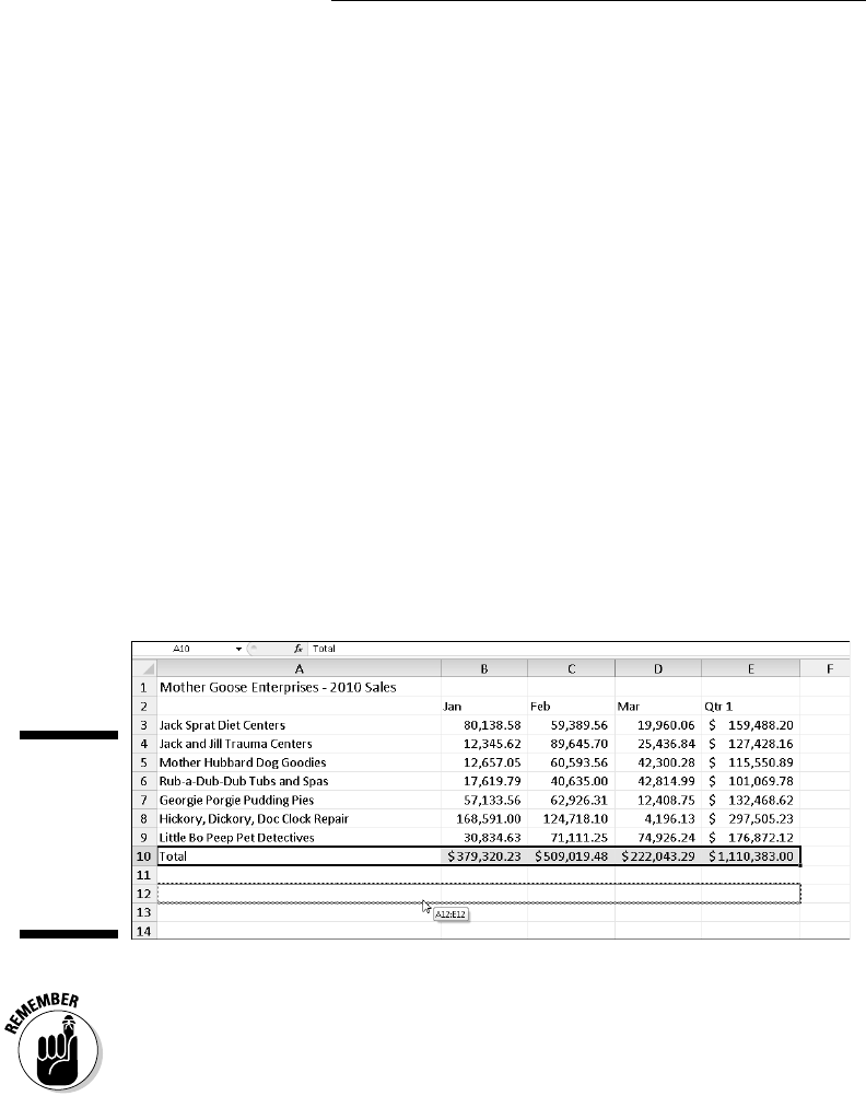
154
Part II: Editing without Tears
3. Drag your selection to its destination.
Drag your selection by depressing and holding down the primary mouse
button — usually the left one — while moving the mouse.
While you drag your selection, you actually move only the outline of
the cell range, and Excel keeps you informed of what the new cell range
address would be (as a kind of drag-and-drop ScreenTip) if you were to
release the mouse button at that location.
Drag the outline until it’s positioned where you want the entries to
appear (as evidenced by the cell range in the drag-and-drop ScreenTip).
4. Release the mouse button.
The cell entries within that range reappear in the new location as soon
as you release the mouse button.
In Figures 4-3 and 4-4, I show how you can drag and drop a cell range. In
Figure 4-3, I select the cell range A10:E10 (containing the quarterly totals)
to move it to row 12 to make room for sales figures for two new companies
(Simple Simon Pie Shoppes and Jack Be Nimble Candlesticks, which hadn’t
been acquired when this workbook was first created). In Figure 4-4, you see
the Mother Goose Enterprises – 2010 Sales worksheet right after completing
this move.
Figure 4-3:
Dragging
the cell
selection
to its new
position in a
worksheet.
The arguments for the SUM functions in cell range B13:E13 do not keep pace
with the change — it continues to sum only the values in rows 3 through
9 after the move. However, when you enter the sales figures for these new
enterprises in columns B through C in rows 10, 11, and 12, Excel shows off
its smarts and updates the formulas in row 13 to include the new entries. For
example, the SUM(B3:B9) formula in B13 magically becomes SUM(B3:B12).
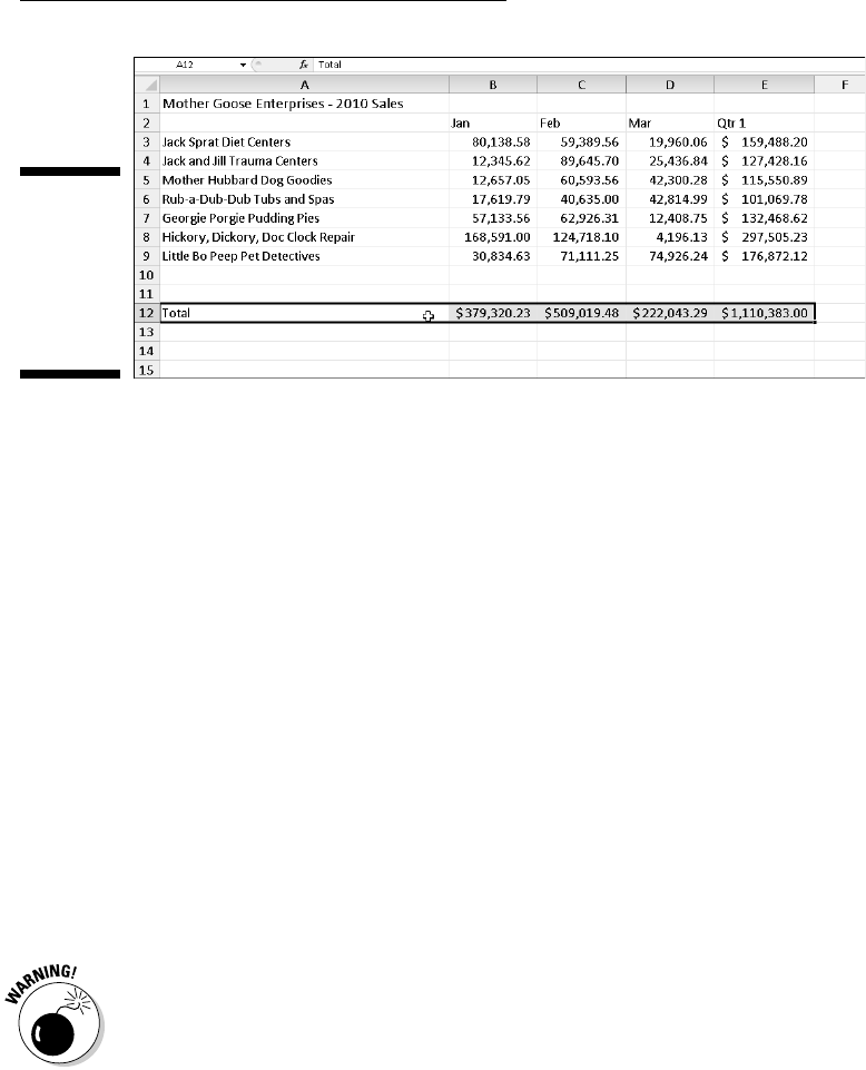
155
Chapter 4: Going Through Changes
Figure 4-4:
A worksheet
after drop-
ping the cell
selection
into its new
place.
Copies, drag-and-drop style
What if you want to copy rather than drag and drop a cell range? Suppose
that you need to start a new table in rows farther down the worksheet, and
you want to copy the cell range with the formatted title and column headings
for the new table. To copy the formatted title range in the sample worksheet,
follow these steps:
1. Select the cell range.
In the case of Figures 4-3 and 4-4, that’s cell range A1:E2.
2. Hold the Ctrl key down while you position the mouse pointer on an
edge of the selection (that is, the expanded cell cursor).
The pointer changes from a thick, shaded cross to an arrowhead with a
+ (plus sign) to the right of it with the drag-and-drop ScreenTip beside
it. The plus sign next to the pointer is your signal that drag and drop will
copy the selection rather than move it.
3. Drag the cell-selection outline to the place where you want the copy to
appear and release the mouse button.
If, when using drag and drop to move or copy cells, you position the outline of
the selection so that it overlaps any part of cells that already contain entries,
Excel displays an alert box that asks whether you want to replace the contents
of the destination cells. To avoid replacing existing entries and to abort the
entire drag-and-drop mission, click the Cancel button in this alert box. To go
ahead and exterminate the little darlings, click OK or press Enter.

156
Part II: Editing without Tears
Insertions courtesy of drag and drop
Like the Klingons of Star Trek fame, spreadsheets, such as Excel, never take
prisoners. When you place or move a new entry into an occupied cell, the
new entry completely replaces the old as though the old entry never existed
in that cell.
To insert the cell range you’re moving or copying within a populated region
of the worksheet without wiping out existing entries, hold down the Shift key
while you drag the selection. (If you’re copying, you have to get ambitious
and hold down both the Shift and Ctrl keys at the same time!)
With the Shift key depressed while you drag, instead of a rectangular outline
of the cell range, you get an I-beam shape that shows where the selection will
be inserted if you release the mouse button along with the address of the cell
range (as a kind of Insertion ScreenTip). When you move the I-beam shape,
notice that it wants to attach itself to the column and row borders while you
move it. After you position the I-beam at the column or row border where
you want to insert the cell range, release the mouse button. Excel inserts
the cell range, moving the existing entries to neighboring blank cells (out of
harm’s way).
When inserting cells with drag and drop, it may be helpful to think of the
I-beam shape as a pry bar that pulls apart the columns or rows along the axis
of the I. Also, sometimes after moving a range to a new place in the worksheet,
instead of the data appearing, you see only #######s in the cells. (Excel 2010
doesn’t automatically widen the new columns for the incoming data as it does
when formatting the data.) Remember that the way to get rid of the #######s
in the cells is by widening those troublesome columns enough to display all
the data-plus-formatting; and the easiest way to do this kind of widening is by
double-clicking the right border of the column.
I held down the Shift key just as you said . . .
Drag and drop in Insert mode is one of Excel’s
most finicky features. Sometimes you can do
everything just right and still get the alert box
warning you that Excel is about to replace exist-
ing entries instead of pushing them aside. When
you see this alert box, always click the Cancel
button! Fortunately, you can insert things with
the Insert commands without worrying about
which way the I-beam selection goes (see the
“Staying In Step with Insert” section, later in
this chapter).
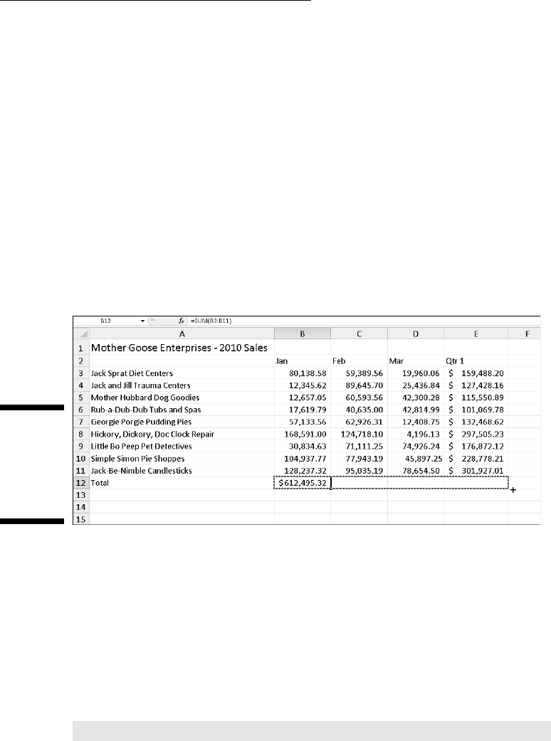
157
Chapter 4: Going Through Changes
Formulas on AutoFill
Copying with drag and drop (by holding down the Ctrl key) is useful when
you need to copy a bunch of neighboring cells to a new part of the work-
sheet. Frequently, however, you just need to copy a single formula that you
just created to a bunch of neighboring cells that need to perform the same
type of calculation (such as totaling columns of figures). This type of formula
copy, although quite common, can’t be done with drag and drop. Instead, use
the AutoFill feature (read about this in Chapter 2) or the Copy and Paste com-
mands. (See the section “Cut and paste, digital style” later in this chapter.)
Here’s how you can use AutoFill to copy one formula to a range of cells. In
Figure 4-5, you can see the Mother Goose Enterprises – 2010 Sales worksheet
with all the companies but this time with only one monthly total in row 12,
which is in the process of being copied through cell E12.
Figure 4-5:
Copying
a formula
to a cell
range with
AutoFill.
Figure 4-6 shows the worksheet after dragging the fill handle in cell B12 to
select the cell range C12:E12 (where this formula should be copied).
Relatively speaking
Figure 4-6 shows the worksheet after the formula in a cell is copied to the cell
range C12:E12 and cell B12 is active. Notice how Excel handles the copying of
formulas. The original formula in cell B12 is as follows:
=SUM(B3:B11)
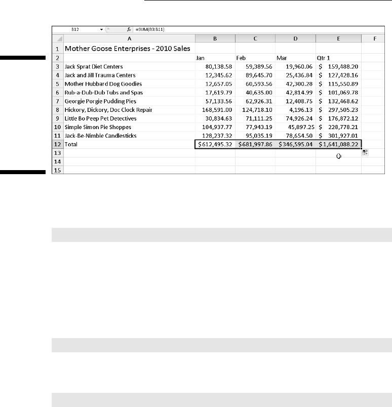
158
Part II: Editing without Tears
Figure 4-6:
The work-
sheet after
copying
the formula
totaling the
monthly
(and quar-
terly) sales.
When the original formula is copied to cell C12, Excel changes the formula
slightly so that it looks like this:
=SUM(C3:C11)
Excel adjusts the column reference, changing it from B to C, because I copied
from left to right across the rows.
When you copy a formula to a cell range that extends down the rows, Excel
adjusts the row numbers in the copied formulas rather than the column
letters to suit the position of each copy. For example, cell E3 in the Mother
Goose Enterprises – 2010 Sales worksheet contains the following formula:
=SUM(B3:D3)
When you copy this formula to cell E4, Excel changes the copy of the formula
to the following:
=SUM(B4:D4)
Excel adjusts the row reference to keep current with the new row 4 position.
Because Excel adjusts the cell references in copies of a formula relative to the
direction of the copying, the cell references are known as relative cell references.
Some things are absolutes!
All new formulas you create naturally contain relative cell references unless
you say otherwise. Because most copies you make of formulas require adjust-
ments of their cell references, you rarely have to give this arrangement a
second thought. Then, every once in a while, you come across an exception
that calls for limiting when and how cell references are adjusted in copies.
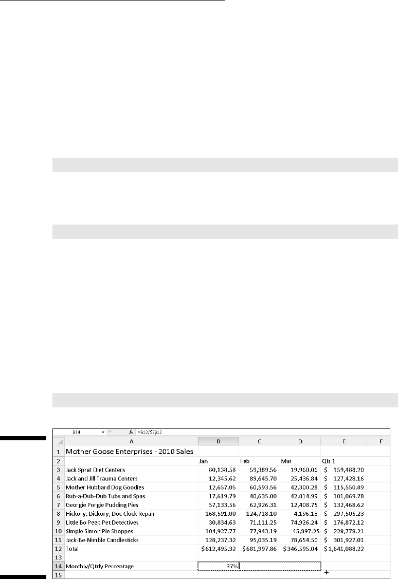
159
Chapter 4: Going Through Changes
One of the most common of these exceptions is when you want to compare
a range of different values with a single value. This happens most often when
you want to compute what percentage each part is to the total. For example, in
the Mother Goose Enterprises – 2010 Sales worksheet, you encounter this situ-
ation in creating and copying a formula that calculates what percentage each
monthly total (in the cell range B14:D14) is of the quarterly total in cell E12.
Suppose that you want to enter these formulas in row 14 of the Mother Goose
Enterprises – 2010 Sales worksheet, starting in cell B14. The formula in cell
B14 for calculating the percentage of the January-sales-to-first-quarter-total is
very straightforward:
=B12/E12
This formula divides the January sales total in cell B12 by the quarterly total
in E12 (what could be easier?). Look, however, at what would happen if you
dragged the fill handle one cell to the right to copy this formula to cell C14:
=C12/F12
The adjustment of the first cell reference from B12 to C12 is just what the
doctor ordered. However, the adjustment of the second cell reference from
E12 to F12 is a disaster. Not only do you not calculate what percentage the
February sales in cell C12 are of the first quarter sales in E12, but you also
end up with one of those horrible #DIV/0! error things in cell C14.
To stop Excel from adjusting a cell reference in a formula in any copies you
make, convert the cell reference from relative to absolute. You do this by
pressing the function key F4, after you put Excel in Edit mode (F2). Excel
indicates that you make the cell reference absolute by placing dollar signs
in front of the column letter and row number. For example, in Figure 4-7, cell
B14 contains the correct formula to copy to the cell range C14:D14:
=B12/$E$12
Figure 4-7:
Copying the
formula for
computing
the ratio of
monthly to
quarterly
sales with
an absolute
cell
reference.
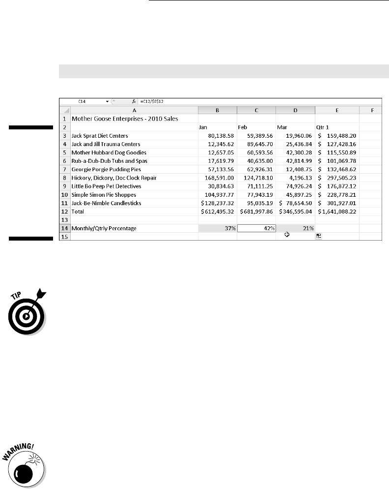
160
Part II: Editing without Tears
Look at the worksheet after this formula is copied to the range C14:D14
with the fill handle and cell C14 is selected (see Figure 4-8). Notice that the
Formula bar shows that this cell contains the following formula:
=C12/$E$12
Figure 4-8:
The work-
sheet after
copying the
formula
with the
absolute
cell
reference.
Because E12 was changed to $E$12 in the original formula, all the copies have
this same absolute (non-changing) reference.
If you goof up and copy a formula where one or more of the cell references
should have been absolute but you left them all relative, edit the original for-
mula as follows:
1. Double-click the cell with the formula or press F2 to edit it.
2. Position the insertion point somewhere on the reference you want to
convert to absolute.
3. Press F4.
4. When you finish editing, click the Enter button on the Formula bar
and then copy the formula to the messed-up cell range with the fill
handle.
Be sure to press F4 only to change a cell reference to completely absolute as
I describe earlier. If you press the F4 function key a second time, you end up
with a so-called mixed reference, where only the row part is absolute and the
column part is relative (as in E$12). If you then press F4 again, Excel comes up
with another type of mixed reference, where the column part is absolute and
the row part is relative (as in $E12). If you go on and press F4 yet again, Excel
changes the cell reference back to completely relative (as in E12). After you’re
back where you started, you can continue to use F4 to cycle through this same
set of cell reference changes all over again.

161
Chapter 4: Going Through Changes
Cut and paste, digital style
Instead of using drag and drop or AutoFill, you can use the old standby Cut,
Copy, and Paste commands to move or copy information in a worksheet.
These commands use the Office Clipboard as a kind of electronic halfway
house where the information you cut or copy remains until you decide to
paste it somewhere. Because of this Clipboard arrangement, you can use
these commands to move or copy information to any other workbook open
in Excel or even to other programs running in Windows (such as a Word 2010
document).
To move a cell selection with Cut and Paste, follow these steps:
1. Select the cells you want to move.
2. Click the Cut command button in the Clipboard group on the Home
tab (the button with the scissors icon).
If you prefer, you can choose Cut by pressing Ctrl+X.
Whenever you choose the Cut command in Excel, the program sur-
rounds the cell selection with a marquee (a dotted line that travels
around the cells’ outline) and displays the following message on the
Status bar:
Select destination and press ENTER or choose Paste
3. Move the cell cursor to the new range to which you want the informa-
tion moved, or click the cell in the upper-left corner of the new range.
4. Press Enter to complete the move operation.
If you’re feeling ambitious, click the Paste command button in the
Clipboard group on the Home tab or press Ctrl+V.
Notice that when you indicate the destination range, you don’t have to select
a range of blank cells that matches the shape and size of the cell selection
you’re moving. Excel needs to know only the location of the cell in the upper-
left corner of the destination range to figure out where to put the rest of the
cells.
Copying a cell selection with the Copy and Paste commands follows an iden-
tical procedure to the one you use with the Cut and Paste commands. After
selecting the range to copy, you can get the information into the Clipboard
by clicking the Copy button on the Ribbon’s Home tab, choosing Copy from
the cell’s shortcut menu, or pressing Ctrl+C.

162
Part II: Editing without Tears
Paste it again, Sam . . .
An advantage to copying a selection with the Copy and Paste commands and
the Clipboard is that you can paste the information multiple times. Just make
sure that, instead of pressing Enter to complete the first copy operation, you
click the Paste button on the Home tab of the Ribbon or press Ctrl+V.
When you use the Paste command to complete a copy operation, Excel
copies the selection to the range you designate without removing the mar-
quee from the original selection. This is your signal that you can select
another destination range (in either the same or a different document).
After you select the first cell of the next range where you want the selection
copied, choose the Paste command again. You can continue in this manner,
pasting the same selection to your heart’s content. When you make the last
copy, press Enter instead of choosing the Paste command button or press-
ing Ctrl+V. If you forget and choose Paste, get rid of the marquee around the
original cell range by pressing the Esc key.
Keeping pace with Paste Options
Right after you click the Paste button on the Home tab of the Ribbon or press
Ctrl+V to paste cell entries that you copy (not cut) to the Clipboard, Excel
displays a Paste Options button with the label, (Ctrl), to its immediate right
at the end of the pasted range. When you click this drop-down button or
press the Ctrl key, a palette similar to the one shown in Figure 4-9 appears
with three groups of buttons (Paste, Paste Values, and Other Paste Options).
Figure 4-9:
Clicking
the Paste
Options
button or
pressing
the Ctrl
key after
complet-
ing a paste
operation
gives you
this palette
of paste
options.
No borders
Values
Keep source
column widths
Formulas
Paste
Formula & number formatting
Keep source formatting
Transpose
Linked picture
Formatting
Picture
Paste link
Values & source formatting
Values & number formatting

163
Chapter 4: Going Through Changes
You can use these paste options to control or restrict the type of content and
formatting that’s included in the pasted cell range. The paste options (com-
plete with the hot key sequences you can type to select them) on the Paste
Options palette include:
✓ Paste (P): Excel pastes all the stuff in the cell selection (formulas, for-
matting, you name it).
✓ Formulas (F): Excel pastes all the text, numbers, and formulas in the cur-
rent cell selection without their formatting.
✓ Formulas & Number Formatting (O): Excel pastes the number formats
assigned to the copied values along with their formulas.
✓ Keep Source Formatting (K): Excel copies the formatting from the origi-
nal cells and pastes this into the destination cells (along with the copied
entries).
✓ No Borders (B): Excel pastes all the stuff in the cell selection without
copying any borders applied to its cell range.
✓ Keep Source Column Widths (W): Excel makes the width of the columns
in the destination range the same as those in the source range when it
copies their cell entries.
✓ Transpose (T): Excel changes the orientation of the pasted entries.
For example, if the original cells’ entries run down the rows of a single
column of the worksheet, the transposed pasted entries will run across
the columns of a single row.
✓ Values (V): Excel pastes only the calculated results of any formulas in
the source cell range.
✓ Values & Number Formatting (A): Excel pastes the calculated results of
any formulas along with all the formatting assigned to the labels, values,
and formulas in the source cell range into the destination range. This
means that all the labels and values in the destination range appear for-
matted just like the source range even though all the original formulas
are lost and only the calculated values are retained.
✓ Values & Source Formatting (E): Excel pastes the calculated results of
any formulas along with all formatting assigned to the source cell range.
✓ Formatting (R): Excel pastes only the formatting (and not the entries)
copied from the source cell range to the destination range.
✓ Paste Link (N): Excel creates linking formulas in the destination range
so that any changes that you make to the entries in cells in the source
range are immediately brought forward and reflected in the correspond-
ing cells of the destination range.
✓ Picture (U): Excel pastes only the pictures in the copied cell selection.
✓ Linked Picture (I): Excel pastes a link to the pictures in the copied cell
selection.
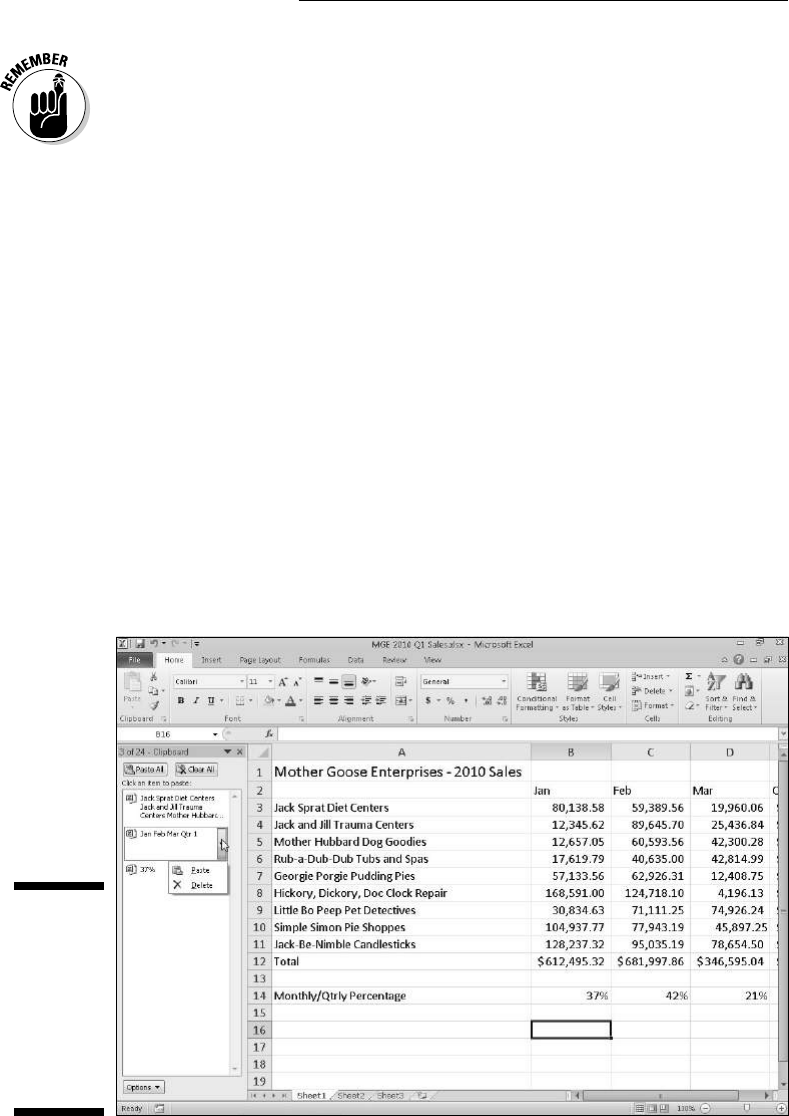
164
Part II: Editing without Tears
The options that appear on the Paste Options palette are context sensitive. This
means that the particular paste options available on the palette depend directly
upon the type of cell entries previously copied to the Office Clipboard.
Additionally, you can access this same palette of paste options by clicking the
drop-down button that appears directly beneath the Paste button on the Ribbon
instead of clicking the Paste Options button that appears at the end of the
pasted range in the worksheet or pressing the Ctrl key on your keyboard.
Paste it from the Clipboard task pane
The Clipboard can store multiple cuts and copies from any program running
under Windows not just Excel. In Excel, this means that you can continue to
paste stuff from the Clipboard into a workbook even after finishing a move or
copy operation (even when you do so by pressing the Enter key rather than
using the Paste command).
To open the Clipboard in its own task pane to the immediate left of the
Worksheet area (see Figure 4-10), click the dialog box launcher in the lower-
right corner of the Clipboard group on the Ribbon’s Home tab.
To paste an item from the Office Clipboard into a worksheet other than the one
with the data last cut or copied onto it, click the item in the Clipboard task pane
to paste it into the worksheet starting at the current position of the cell cursor.
Figure 4-10:
The
Clipboard
task pane
appears on
the left side
of the Excel
Worksheet
area.

165
Chapter 4: Going Through Changes
You can paste all the items stored in the Office Clipboard into the current
worksheet by clicking the Paste All button at the top of the Clipboard task
pane. To clear the Office Clipboard of all the current items, click the Clear All
button. To delete only a particular item from the Office Clipboard, position
the mouse pointer over the item in the Clipboard task pane until its drop-
down button appears. Click this drop-down button, and then choose Delete
from the pop-up menu (refer to Figure 4-10).
To have the Clipboard task pane appear automatically after making two
cuts or copies to the Clipboard in an Excel workbook, click the Show Office
Clipboard Automatically option on the task pane’s Options button menu.
To open the Clipboard task pane in the Excel program window by pressing
Ctrl+CC, click Show Office Clipboard When Ctrl+C Pressed Twice on the task
pane’s Options button. Pressing Ctrl+CC only opens the task pane. You still
have to click the Close button on the Office Clipboard to close the task pane.
So what’s so special about Paste Special?
Normally, unless you fool around with the Paste Options (see the section
“Keeping pace with Paste Options” earlier in this chapter), Excel copies all the
information in the range of cells you selected: formatting, as well the formulas,
text, and other values you enter. You can use the Paste Special command to
specify which entries and formatting to use in the current paste operation. Many
of the Paste Special options are also available on the Paste Options palette.
To paste particular parts of a cell selection while discarding others, click the
drop-down button that appears at the bottom of the Paste command button
on the Ribbon’s Home tab. Then, click Paste Special on its drop-down menu
to open the Paste Special dialog box shown in Figure 4-11.
Figure 4-11:
Use the
options in
the Paste
Special dia-
log box to
control what
part of the
copied cell
selection to
include in
the paste
operation.

166
Part II: Editing without Tears
The options in the Paste Special dialog box include:
✓ All to paste all the stuff in the cell selection (formulas, formatting, you
name it).
✓ Formulas to paste all the text, numbers, and formulas in the current cell
selection without their formatting.
✓ Values to convert formulas in the current cell selection to their calcu-
lated values.
✓ Formats to paste only the formatting from the current cell selection,
leaving the cell entries in the dust.
✓ Comments to paste only the notes that you attach to their cells (kind of
like electronic self-stick notes — see Chapter 6 for details).
✓ Validation to paste only the data validation rules into the cell range
that you set up with the Data Validation command (which enables you
to set what value or range of values is allowed in a particular cell or cell
range).
✓ All Using Source Theme to paste all the information plus the cell styles
applied to the cells.
✓ All Except Borders to paste all the stuff in the cell selection without
copying any borders you use there.
✓ Column Widths to apply the column widths of the cells copied to the
Clipboard to the columns where the cells are pasted.
✓ Formulas and Number Formats to include the number formats assigned
to the pasted values and formulas.
✓ Values and Number Formats to convert formulas to their calculated
values and include the number formats you assign to all the pasted
values.
✓ All Merging Conditional Formats to paste Conditional Formatting into
the cell range.
✓ None to have Excel perform no mathematical operation between the
data entries you cut or copy to the Clipboard and the data entries in the
cell range where you paste.
✓ Add to add the data you cut or copy to the Clipboard and the data
entries in the cell range where you paste.
✓ Subtract to subtract the data you cut or copy to the Clipboard from the
data entries in the cell range where you paste.
✓ Multiply to multiply the data you cut or copy to the Clipboard by the
data entries in the cell range where you paste.
✓ Divide to divide the data you cut or copy to the Clipboard by the data
entries in the cell range where you paste.

167
Chapter 4: Going Through Changes
✓ Skip Blanks check box when you want Excel to paste everywhere except
for any empty cells in the incoming range. In other words, a blank cell
cannot overwrite your current cell entries.
✓ Transpose check box when you want Excel to change the orientation of
the pasted entries. For example, if the original cells’ entries run down
the rows of a single column of the worksheet, the transposed pasted
entries will run across the columns of a single row.
✓ Paste Link button when you’re copying cell entries and you want to
establish a link between copies you’re pasting and the original entries.
That way, changes to the original cells automatically update in the
pasted copies.
Let’s Be Clear about Deleting Stuff
No discussion about editing in Excel would be complete without a section on
getting rid of the stuff you put into cells. You can perform two kinds of dele-
tions in a worksheet:
✓ Clearing a cell: Clearing just deletes or empties the cell’s contents with-
out removing the cell from the worksheet, which would alter the layout
of the surrounding cells.
✓ Deleting a cell: Deleting gets rid of the whole kit and caboodle — cell
structure along with all its contents and formatting. When you delete a
cell, Excel has to shuffle the position of entries in the surrounding cells
to plug up any gaps made by the action.
Sounding the all clear!
To get rid of just the contents of a cell selection rather than delete the cells
and their contents, select the range of cells to clear and then simply press
the Delete key.
If you want to get rid of more than just the contents of a cell selection,
click the Clear button (the one with the eraser) in the Editing group on the
Ribbon’s Home tab and then click one of the following options on its drop-
down menu:
✓ Clear All: Gets rid of all formatting and notes, as well as entries in the
cell selection (Alt+HEA).
✓ Clear Formats: Deletes only the formatting from the cell selection with-
out touching anything else (Alt+HEF).

168
Part II: Editing without Tears
✓ Clear Contents: Deletes only the entries in the cell selection just like
pressing the Delete key (Alt+HEC).
✓ Clear Comments: Removes the notes in the cell selection but leaves
everything else behind (Alt+HEM).
✓ Clear Hyperlinks: Removes the active hyperlinks (see Chapter 12) in the
cell selection but leaves its descriptive text (Alt+HEL).
Get these cells outta here!
To delete the cell selection rather than just clear out its contents, select
the cell range, click the drop-down button attached to the Delete command
button in the Cells group of the Home tab, and then click Delete Cells on the
drop-down menu (or press Alt+HDD). The Delete dialog box opens, showing
options for filling in the gaps created when the cells currently selected are
blotted out of existence:
✓ Shift Cells Left: This default option moves entries from neighboring col-
umns on the right to the left to fill in gaps created when you delete the
cell selection by clicking OK or pressing Enter.
✓ Shift Cells Up: Select this to move entries up from neighboring rows
below.
✓ Entire Row: Select this to remove all the rows in the current cell
selection.
✓ Entire Columns: Select this to delete all the columns in the current cell
selection.
If you know that you want to shift the remaining cells to the left after deleting
the cells in the current selection, you can simply click the Delete command
button on the Home tab of the Ribbon. (This is the same thing as opening the
Delete dialog box and then clicking OK when the default Shift Cells Left button
is selected.
To delete an entire column or row from the worksheet, you can select the
column or row on the workbook window frame, right-click the selection, and
then click Delete from the column’s or row’s shortcut menu.
You can also delete entire columns and rows selected in the worksheet by
clicking the drop-down button attached to the Delete command button on
the Ribbon’s Home tab and then clicking the Delete Sheet Columns (Alt+HDC)
option or the Delete Sheet Rows option (Alt+HDR) on the drop-down menu.

169
Chapter 4: Going Through Changes
Deleting entire columns and rows from a worksheet is risky business unless
you are sure that the columns and rows in question contain nothing of value.
Remember, when you delete an entire row from the worksheet, you delete all
information from column A through XFD in that row (and you can see only a
very few columns in this row). Likewise, when you delete an entire column
from the worksheet, you delete all information from row 1 through 1,048,576 in
that column.
Staying in Step with Insert
For those inevitable times when you need to squeeze new entries into an
already populated region of the worksheet, you can insert new cells in the
area rather than go through all the trouble of moving and rearranging sev-
eral individual cell ranges. To insert a new cell range, select the cells (many
of which are already occupied) where you want the new cells to appear and
then click the drop-down attached to the Insert command button in the Cells
group of the Home tab and then click Insert Cells on the drop-down menu (or
press Alt+HII). The Insert dialog box opens with the following option buttons:
✓ Shift Cells Right: Select this to shift existing cells to the right to make
room for the ones you want to add before clicking OK or pressing Enter.
✓ Shift Cells Down: Use this default to instruct the program to shift exist-
ing entries down before clicking OK or pressing Enter.
✓ Entire Row or Entire Column: When you insert cells with the Insert
dialog box, you can insert complete rows or columns in the cell range
by selecting either of these radio buttons. You can also select the row
number or column letter on the frame before you choose the Insert
command.
If you know that you want to shift the existing cells to the right to make room
for the newly inserted cells, you can simply click the Insert command button
on the Ribbon’s Home tab (this is the same thing as opening the Insert dialog
box and then clicking OK when the Shift Cells Right button is selected).
Remember that you can also insert entire columns and rows in a worksheet by
right-clicking the selection and then clicking Insert on the column’s or row’s
shortcut menu.
As when you delete whole columns and rows, inserting entire columns and
rows affects the entire worksheet, not just the part you see. If you don’t know
what’s out in the hinterlands of the worksheet, you can’t be sure how the
insertion will affect — perhaps even sabotage — stuff (especially formulas) in
the other unseen areas. I suggest that you scroll all the way out in both direc-
tions to make sure that nothing’s out there.
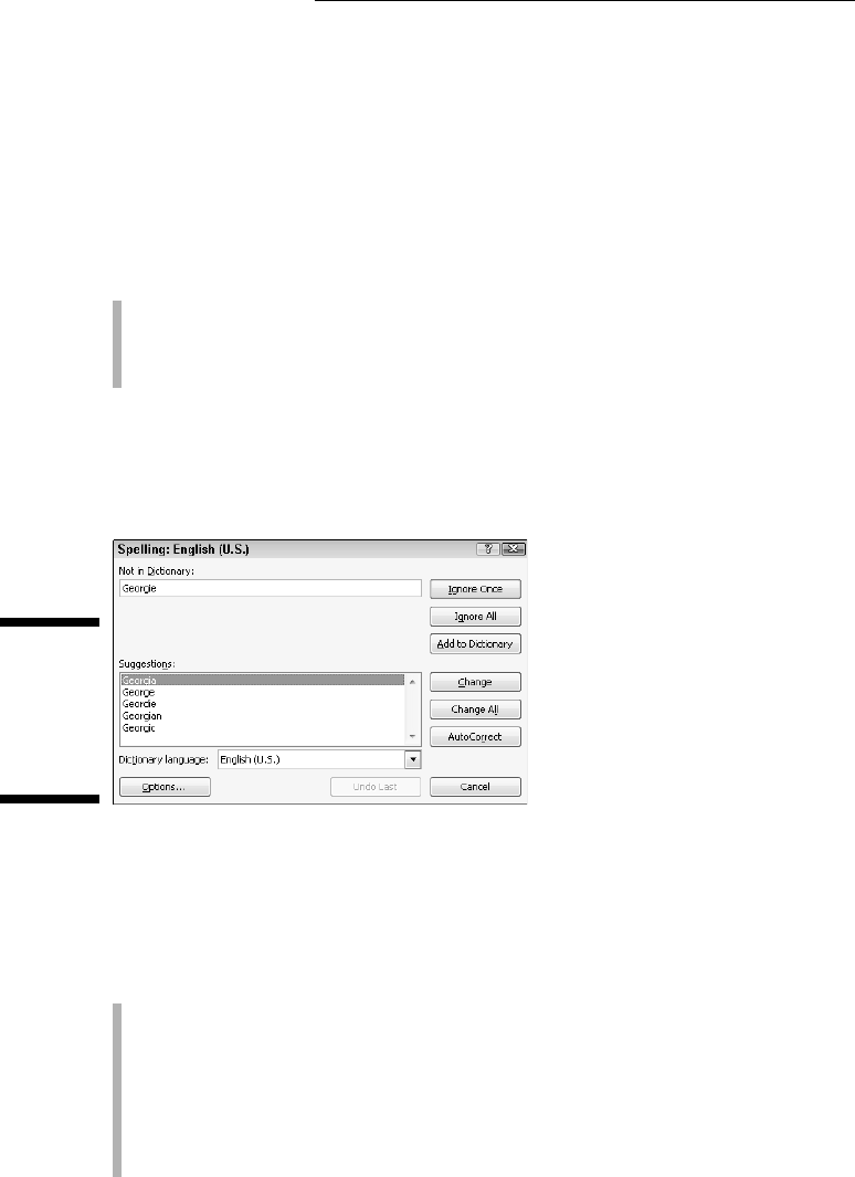
170
Part II: Editing without Tears
Stamping Out Your Spelling Errors
If you’re as good a speller as I am, you’ll be relieved to know that Excel 2010
has a built-in spell checker that can catch and remove all those embarrass-
ing little spelling errors. With this in mind, you no longer have any excuse for
putting out worksheets with typos in the titles or headings.
To check the spelling in a worksheet, you have the following options:
✓ Click the Spelling command button on the Ribbon’s Review tab
✓ Press Alt+RS
✓ Press F7
Any way you do it, Excel begins checking the spelling of all text entries in the
worksheet. When the program comes across an unknown word, it displays
the Spelling dialog box, similar to the one shown in Figure 4-12.
Figure 4-12:
Check your
spelling
from the
Spelling dia-
log box.
Excel suggests replacements for the unknown word shown in the Not in
Dictionary text box with a likely replacement in the Suggestions list box
of the Spelling dialog box. If that replacement is incorrect, you can scroll
through the Suggestions list and click the correct replacement. Use the
Spelling dialog box options as follows:
✓ Ignore Once and Ignore All: When Excel’s spell check comes across
a word its dictionary finds suspicious but you know is viable, click the
Ignore Once button. If you don’t want the spell checker to bother query-
ing you about this word again, click the Ignore All button.
✓ Add to Dictionary: Click this button to add the unknown (to Excel)
word — such as your name — to a custom dictionary so that Excel
won’t flag it again when you check the spelling in the worksheet later on.

171
Chapter 4: Going Through Changes
✓ Change: Click this button to replace the word listed in the Not in
Dictionary text box with the word Excel offers in the Suggestions list
box.
✓ Change All: Click this button to change all occurrences of this mis-
spelled word in the worksheet to the word Excel displays in the
Suggestions list box.
✓ AutoCorrect: Click this button to have Excel automatically correct this
spelling error with the suggestion displayed in the Suggestions list box
(by adding the misspelling and suggestion to the AutoCorrect dialog
box; for more, read Chapter 2).
✓ Dictionary Language: To switch to another dictionary (such as a United
Kingdom English dictionary, or a French dictionary when checking
French terms in a multilingual worksheet), click this drop-down button
and then select the name of the desired language in the list.
Notice that the Excel spell checker not only flags words not found in its built-
in or custom dictionary but also flags occurrences of double words in a cell
entry (such as total total) and words with unusual capitalization (such as NEw
York instead of New York). By default, the spell checker ignores all words
with numbers and all Internet addresses. If you want it to ignore all words
in uppercase letters as well, click the Options button at the bottom of the
Spelling dialog box, and then select the Ignore Words in UPPERCASE check
box before clicking OK.
You can check the spelling of just a particular group of entries by selecting
the cells before you click the Spelling command button on the Review tab of
the Ribbon or press F7.
Stamping Out Errors with Text to Speech
The good news is that Excel 2010 still supports the Text to Speech feature
introduced in Excel 2003. This feature enables your computer to read aloud
any series of cell entries in the worksheet. By using Text to Speech, you can
check your printed source while the computer reads aloud the values and
labels that you’ve actually entered — a real nifty way to catch and correct
errors that may otherwise escape unnoticed.
The Text to Speech translation feature requires no prior training or special
microphones: All that’s required is a pair of speakers or headphones con-
nected to your computer.

172
Part II: Editing without Tears
Now for the bad news: Text to Speech is not available from any of the tabs
on the Ribbon. The only way to access Text to Speech is by adding its Speak
Cells command buttons as custom buttons on a custom tab on the Ribbon or
as custom buttons on the Quick Access toolbar as follows:
1. Click the Customize Quick Access Toolbar button at the very end of
the Quick Access toolbar and then click More Commands on its menu.
The Quick Access Toolbar tab of the Excel Options dialog box opens.
2. Click Commands Not in the Ribbon on the Choose Commands From
drop-down menu and scroll down until you see the Speak Cells com-
mands.
The Text to Speech command buttons include Speak Cells, Speak Cells –
Stop Speaking Cells, Speak Cells by Columns, Speak Cells by Rows, and
Speak Cells on Enter.
3. Click the Speak Cells button in the Choose Commands From list box
on the left and then click the Add button to add it to the bottom of the
Customize Quick Access Toolbar list box on the right.
4. Repeat Step 3 until you’ve added the remaining Text to Speech but-
tons to the Quick Access toolbar: Speak Cells – Stop Speaking Cells,
Speak Cells by Columns, Speak Cells by Rows, and Speak Cells on
Enter.
If you want to reposition the Text to Speech buttons on the Quick
Access toolbar, select each button in the Customize Quick Access
Toolbar list and then move it left on the bar by clicking the Move Up
button or right by clicking Move Down. If you want to set off the Text to
Speech buttons as a separate group on the Quick Access toolbar, add
a vertical separator ahead of the Speak Cells command button (and fol-
lowing the Speak Cells on Enter button if you have buttons not related to
the Text to Speech function that follow on the Quick Access toolbar).
5. Click the OK button to close the Excel Options dialog box.
Figure 4-13 shows the Quick Access toolbar in my Excel 2010 program
window after I moved the toolbar down so that it appears below the Ribbon
and added athe Speak Cells command buttons to it.
After adding the Text to Speech commands as custom Speak Cells buttons
on the Quick Access toolbar, you can use them to corroborate spreadsheet
entries and catch those hard-to-spot errors as follows:
1. Select the cells in the worksheet whose contents you want read aloud
by Text to Speech.
2. Click the Speak Cells custom button on the Quick Access toolbar to
have the computer read the entries in the selected cells.
By default, the Text to Speech feature reads the contents of each cell
in the cell selection by reading down each column and then across the
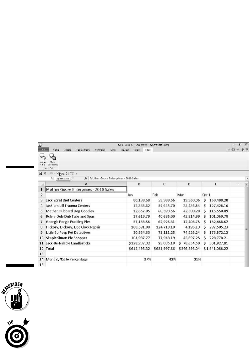
173
Chapter 4: Going Through Changes
rows. If you want Text to Speech to read across the rows and then down
the columns, click the Speak Cells by Rows button on the Quick Access
toolbar (the button with the two opposing horizontal arrows).
3. To have the Text to Speech feature read each cell entry while you
press the Enter key (at which point the cell cursor moves down to
the next cell in the selection), click the Speak Cells on Enter custom
button (the button with the curved arrow Enter symbol) on the Quick
Access toolbar.
As soon as you click the Speak Cells on Enter button, the computer tells
you, “Cells will now be spoken on Enter.” After selecting this option, you
need to press Enter each time that you want to hear an entry read to you.
4. To pause the Text to Speech feature when you’re not using the Speak
Cells on Enter option (Step 3) and you locate a discrepancy between
what you’re reading and what you’re hearing, click the Stop Speaking
button (the Speak Cells group button with the x).
Figure 4-13:
After add-
ing the
Speak Cells
command
buttons to
the Quick
Access tool-
bar, you can
use them
to check
cell entries
audibly.
After you click the Speak Cells on Enter button on the Quick Access toolbar,
the computer speaks only each new cell entry that you complete by pressing
the Enter key (which moves the cell cursor down one row) rather than some
other method, such as clicking the Enter button on the Formula bar or press-
ing the ↓ key.
You can also add any or all the Text to Speech buttons to a custom group on a
custom tab on the Ribbon (for example, the Speak Cells group on the custom
Misc tab in Figure 4-13 contains the Speak Cells and Stop Speaking buttons).

174
Part II: Editing without Tears

Chapter 5
Printing the Masterpiece
In This Chapter
▶ Previewing pages in Page Layout View and printouts in Backstage View
▶ Quick Printing from the Quick Access toolbar
▶ Printing all the worksheets in a workbook
▶ Printing just some of the cells in a worksheet
▶ Changing page orientation
▶ Printing the whole worksheet on a single page
▶ Changing margins for a report
▶ Adding a header and footer to a report
▶ Printing column and row headings as print titles on every page of a report
▶ Inserting page breaks in a report
▶ Printing the formulas in your worksheet
F
or most people, getting data down on paper is what spreadsheets are
all about (all the talk about a so-called paperless office to the contrary).
Everything — all the data entry, all the formatting, all the formula checking,
all the things you do to get a spreadsheet ready — is really just preparation
for printing its information.
In this chapter, you find out just how easy it is to print reports with Excel
2010. Thanks to the program’s new Print panel in Backstage View (Alt+FP), its
Page Layout worksheet view, and its handy Page Layout tab on the Ribbon,
you discover how to produce top-notch reports the first time you send
the document to the printer (instead of the second or even the third time
around).
The only trick to printing a worksheet is getting used to the paging scheme
and learning how to control it. Many of the worksheets you create with Excel
are not only longer than one printed page but also wider. Word processors,
such as Word 2010, page the document only vertically; they won’t let you

176
Part II: Editing without Tears
create a document wider than the page size you’re using. Spreadsheet pro-
grams like Excel 2010, however, often have to break up pages both vertically
and horizontally to print a worksheet document (a kind of tiling of the print
job, if you will).
When breaking a worksheet into pages, Excel first pages the document verti-
cally down the rows in the first columns of the print area (just like a word
processor). After paging the first columns, the program pages down the rows
of the second set of columns in the print area. Excel pages down and then
over until the entire document included in the current print area (which can
include the entire worksheet or just sections) is paged.
When paging the worksheet, Excel doesn’t break up the information within
a row or column. If not all the information in a row will fit at the bottom of
the page, the program moves the entire row to the following page. If not all
the information in a column will fit at the right edge of the page, the program
moves the entire column to a new page. (Because Excel pages down and then
over, the column may not appear on the next page of the report.)
You can deal with such paging problems in several ways, and in this chapter,
you see all of them! After you have these page problems under control, print-
ing is a proverbial piece of cake.
Taking a Gander at the Pages
in Page Layout View
Excel 2010’s Page Layout View gives you instant access to the paging of the
current worksheet. Activate this feature by clicking the Page Layout View
button (the center one) to the immediate left of the Zoom slider on the Status
bar or by clicking the Page Layout View command button on the Ribbon’s
View tab (Alt+WP). As you can see in Figure 5-1, when you switch to Page
Layout View, Excel adds horizontal and vertical rulers to the column letter
and row number headings. In the Worksheet area, this view shows the mar-
gins for each printed page, any headers and footers defined for the report,
and the breaks between each page. (Often, you have to use the Zoom slider
to reduce the screen magnification to display the page breaks on the screen.)
To see all the pages in the active worksheet, drag the slider button in the
Zoom slider on the Status bar to the left until you decrease the screen magnifi-
cation sufficiently to display all the pages of data.
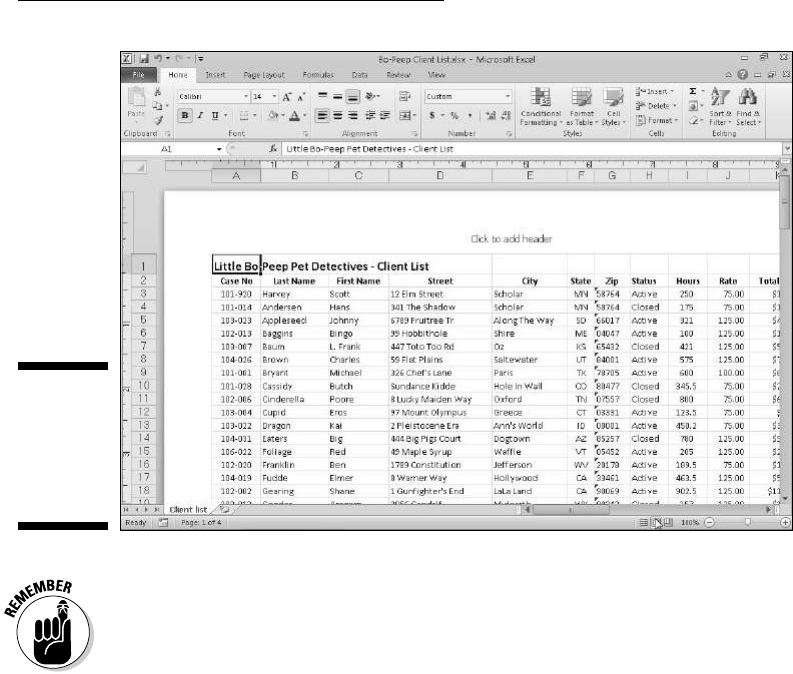
177
Chapter 5: Printing the Masterpiece
Figure 5-1:
Viewing a
spreadsheet
in Page
Layout
View.
Excel displays rulers using the default units for your computer (inches
on a U.S. computer and centimeters on a European machine). To change
the units, open the Advanced tab of the Excel Options dialog box
(File➪Options➪Advanced or Alt+FIA) and then select the appropriate unit
(Inches, Centimeters, or Millimeters) on the Ruler Units drop-down menu in
the Display section.
The Ruler check box on the View tab acts as a toggle switch so that the first
time you click this button, Excel removes the rulers from the Page Layout
View, and the second time you click this button, the program adds them
again.
Checking and Printing a Report
from the Print Panel
To save wasted paper and your sanity, print your worksheet directly from
the Print panel in Backstage View by clicking File➪Print (or simply pressing
Ctrl+P or Ctrl+F2). As you see in Figure 5-2, the Print panel shows you at-a-
glance your current print settings along with a preview of the first page of the
printout.
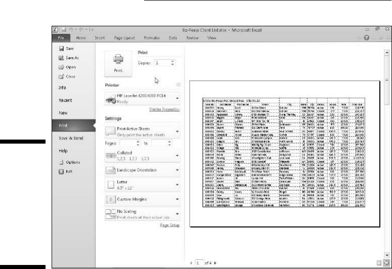
178
Part II: Editing without Tears
Figure 5-2:
The Print
panel in
Backstage
View shows
your current
print set-
tings plus a
preview of
the printout.
You can use the Print Preview feature in the Print panel before you print any
worksheet, section of worksheet, or entire workbook. Because of the pecu-
liarities in paging worksheet data, you often need to check the page breaks
for any report that requires more than one page. The print preview area in
the Print panel shows you exactly how the worksheet data will page when
printed. If necessary, you can return to the worksheet where you can make
changes to the page settings from the Page Layout tab on the Ribbon before
sending the report to the printer when everything looks okay.
When Excel displays a full page in the print preview area, you can barely read
its contents. To increase the view to actual size to verify some of the data, click
the Zoom to Page button in the lower-right corner of the Print panel. Check out
the difference in Figure 5-3 — you can see what the first page of the four-page
report looks like after I zoom in by clicking this Zoom to Page button.
After you enlarge a page to actual size, use the scroll bars to bring new parts
of the page into view in the print preview area. To return to the full-page
view, click the Zoom to Page button a second time to deselect it.
Excel indicates the number of pages in a report at the bottom of the print
preview area. If your report has more than one page, you can view pages
that follow by clicking the Next Page button to the right of the final page
number. To review a page you’ve already seen, back up a page by clicking the
Previous Page button to the left of the first page number. (The Previous Page
button is gray if you’re on the first page.)
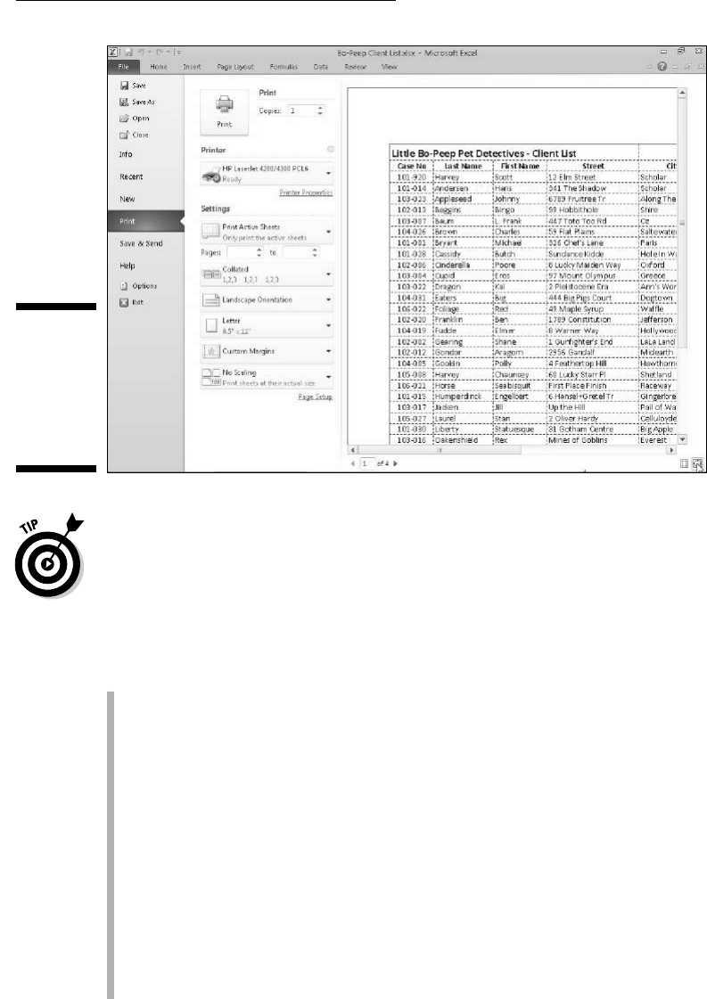
179
Chapter 5: Printing the Masterpiece
Figure 5-3:
Page 1 of a
four-page
report after
clicking the
Zoom to
Page button.
To display markers indicating the current left, right, top and bottom margins
along with the column widths, select the Show Margins check box to the
immediate left of the Zoom to Page button. You can then modify the column
widths as well as the page margins by dragging the appropriate marker (see
“Massaging the margins” later in this chapter for details).
When you finish previewing the report, the Print panel offers you the following
options for changing certain print settings before you send it to the printer:
✓ Print button with the Number of Copies combo box: Use this button to
print the spreadsheet report using the current print settings listed on
the panel. Use the combo box to indicate the number of copies you want
when you need multiple copies printed.
✓ Printer drop-down button: Use this button to select a new printer or
fax to send the spreadsheet report to when more than one device is
installed. (Excel automatically displays the name of the printer that’s
installed as the default printer in Windows.)
✓ Settings drop-down buttons: These include a Print What drop-down button
with attendant Pages combo boxes: Use the Print What drop-down button
to choose between printing only the active (selected) worksheets in the
workbook (the default), the entire workbook, the current cell selection in
the current worksheet, and the currently selected table in the current work-
sheet. Use the combo boxes to restrict what’s printed to just the range of
pages you enter in these boxes or select with their spinner buttons.

180
Part II: Editing without Tears
Beneath the combo boxes, you find drop-down list buttons to print on
both sides of each page in the report, collate the pages of the report,
and switch the page orientation from Portrait (aligned with the short
side) to Landscape (aligned with the long side). Additionally, you can
select a paper size other than the standard 8.5" x 11" letter, and custom-
ize the size of the report’s margins (top, bottom, left, and right, as well
as the margins for any header and footer on the page).
Printing Just the Current Worksheet
As long as you want to use Excel’s default print settings to print all the cells in
the current worksheet, printing in Excel 2010 is a breeze. Simply add the Quick
Print button to the Quick Access toolbar (by clicking the Customize Quick
Access Toolbar button and then clicking Quick Print on its drop-down menu).
After adding the Quick Print button to the Quick Access toolbar, you can use
this button to print a single copy of all the information in the current work-
sheet, including any charts and graphics — but not including comments you
add to cells. (See Chapter 6 for details about adding comments to your work-
sheet and Chapter 10 for details about charts and graphics.)
Understanding and using the print area
Excel includes a special printing feature called
Print Area. Click Print Area➪Set Print Area on
the Ribbon’s Page Layout tab or press Alt+PRS
to define any cell selection on a worksheet as
the print area. After you define the print area,
Excel then prints this cell selection anytime you
print the worksheet (by using either the Quick
Print button, if you’ve added it to the Quick
Access toolbar or by using the File➪Print com-
mand or its Ctrl+P shortcut).
After you define the print area, its cell range
is the only one you can print (regardless of
what other Print What option you select in the
Settings section of the Print panel). That is,
unless you click the Ignore Print Area option at
the very bottom of the Print What drop-down list
or clear the print area. To clear the print area
(and return to the printing defaults that Excel
establishes in the Print dialog box), click Print
Area➪Clear Print Area on the Page Layout tab
or simply press Alt+PRC.
You can also define and clear the print area
from the Sheet tab of the Page Setup dialog
box by clicking the dialog box launcher in the
Page Setup group on the Ribbon’s Page Layout
tab. To define the print area from this dialog
box, click the Print Area text box on the Sheet
tab to insert the cursor and then select the cell
range or ranges in the worksheet (remembering
that you can reduce the Page Setup dialog box
to just this text box by clicking the Print Area
Collapse/Expand button). To clear the print area
from this dialog box, select the cell addresses in
the Print Area text box and press the Delete key.

181
Chapter 5: Printing the Masterpiece
When you click the Quick Print button, Excel routes the print job to the
Windows print queue, which acts like a middleman and sends the job to the
printer. While Excel sends the print job to the print queue, Excel displays a
Printing dialog box to inform you of its progress (displaying such updates as
Printing Page 2 of 3). After this dialog box disappears, you are free to go back
to work in Excel. To stop the printing while the job is still being sent to the
print queue, click the Cancel button in the Printing dialog box.
If you don’t realize that you want to cancel the print job until after Excel
finishes shipping it to the print queue (that is, while the Printing dialog box
appears onscreen), you must:
1. Click the printer icon in the Notification area at the far right of the
Windows taskbar (to the immediate left of the current time) with the
secondary mouse button to open its shortcut menu.
This printer icon displays the ScreenTip 1 document(s) pending
for so-and-so. For example, when I’m printing, this message reads 1
document(s) pending for Greg when I position the mouse pointer over the
printer icon.
2. Right-click the printer icon and then select the Open All Active
Printers command from its shortcut menu.
This opens the dialog box for the printer with the Excel print job in its
queue (as described under the Document Name heading in the list box).
3. Select the Excel print job that you want to cancel in the list box of
your printer’s dialog box.
4. Choose Document➪Cancel from the menu bar and then click Yes to
confirm you want to cancel the print job.
5. Wait for the print job to disappear from the queue in the printer’s
dialog box and then click the Close button to return to Excel.
My Page Was Set Up!
About the only thing the slightest bit complex in printing a worksheet is figur-
ing out how to get the pages right. Fortunately, the command buttons in the
Page Setup group on the Ribbon’s Page Layout tab give you a great deal of
control over what goes on which page.
Three groups of buttons on the Page Layout tab help you get your page set-
tings exactly as you want them. The Page Setup group, the Scale to Fit group,
and the Sheet Options group are described in the following sections.

182
Part II: Editing without Tears
To see the effect of changes you make in the Worksheet area, put the work-
sheet into Page Layout View by clicking the Page Layout button on the Status
bar while you work with the command buttons in the Page Setup, Scale to Fit,
and Sheet Options groups on the Page Layout tab of the Ribbon.
Using the buttons in the Page Setup group
The Page Setup group of the Page Layout tab contains the following impor-
tant command buttons:
✓ Margins button to select one of three preset margins for the report or
to set custom margins on the Margins tab of the Page Setup dialog box.
(See “Massaging the margins” that follows in this chapter.)
✓ Orientation button to switch between Portrait and Landscape mode for
printing. (See the “Getting the lay of the landscape” section, later in this
chapter.)
✓ Size button to select one of the preset paper sizes, set a custom size, or
change the printing resolution or page number on the Page tab of the
Page Setup dialog box.
✓ Print Area button to set and clear the print area. (See the nearby
“Understanding and using the print area” sidebar.)
✓ Breaks button to insert or remove page breaks. (See “Solving Page Break
Problems” later in this chapter.)
✓ Background button to open the Sheet Background dialog box where you
can select a new graphic image or photo to use as a background for the
current worksheet. (This button changes to Delete Background as soon
as you select a background image.)
✓ Print Titles button to open the Sheet tab of the Page Setup dialog box
where you can define rows of the worksheet to repeat at the top and col-
umns of the worksheet to repeat at the left as print titles for the report.
(See “Putting out the print titles” later in this chapter.)
Massaging the margins
The Normal margin settings that Excel applies to a new report uses standard
top, bottom, left, and right margins of
3
⁄4 inch with just over a
1
⁄4 inch separat-
ing the header and footer from the top and bottom margin, respectively.
In addition to the Normal margin settings, the program enables you to select
two other standard margins from the Margins button’s drop-down menu:
✓ Wide margins with 1-inch top, bottom, left, and right margins and
1
⁄2
inch separating the header and footer from the top and bottom margin,
respectively.

183
Chapter 5: Printing the Masterpiece
✓ Narrow margins with a top and bottom margin of
3
⁄4 inch and a left and
right margin of
1
⁄4 inch with 0.3 inch separating the header and footer
from the top and bottom margin, respectively.
Frequently, you find yourself with a report that takes up a full printed page
and then just enough to spill over onto a second, mostly empty, page. To
squeeze the last column or the last few rows of the worksheet data onto Page
1, try selecting Narrow on the Margins button’s drop-down menu.
If that doesn’t do it, you can try manually adjusting the margins for the report
from the Margins tab of the Page Setup dialog box or by dragging the margin
markers in the preview area of the Print panel in the Backstage View (Press
Ctrl+P and click the Show Margins button). To get more columns on a page,
try reducing the left and right margins. To get more rows on a page, try
reducing the top and bottom margins.
To open the Margins tab of the Page Setup dialog box (shown in Figure 5-4),
click Custom Margins on the Margins button’s drop-down menu. There, enter
the new settings in the Top, Bottom, Left, and Right text boxes — or select
the new margin settings with their respective spinner buttons.
Figure 5-4:
Adjust your
report mar-
gins from
the Margins
tab in the
Page Setup
dialog box.
Select one or both Center on Page options in the Margins tab of the Page Setup
dialog box (refer to Figure 5-4) to center a selection of data (that takes up less
than a full page) between the current margin settings. In the Center on Page
section, select the Horizontally check box to center the data between the left
and right margins. Select the Vertically check box to center the data between
the top and bottom margins.
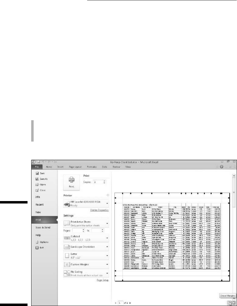
184
Part II: Editing without Tears
When you select the Show Margins button in the Print panel in the Backstage
View (Ctrl+P) to modify the margin settings directly, you can also massage
the column widths as well as the margins. (Refer to Figure 5-5.) To change
one of the margins, position the mouse pointer on the desired margin marker
(the pointer shape changes to a double-headed arrow) and drag the marker
with your mouse in the appropriate direction. When you release the mouse
button, Excel redraws the page, using the new margin setting. You may gain
or lose columns or rows, depending on what kind of adjustment you make.
Changing the column widths is the same story: Drag the column marker to
the left or right to decrease or increase the width of a particular column.
Getting the lay of the landscape
The drop-down menu attached to the Orientation button in the Page Setup
group of the Ribbon’s Page Layout tab contains two options:
✓ Portrait (the default) where the printing runs parallel to the short edge
of the paper
✓ Landscape where the printing runs parallel to the long edge of the paper
Figure 5-5:
Drag a
marker to
adjust its
margin in
the page
preview
area of
the Print
panel when
the Show
Margins
button is
selected.
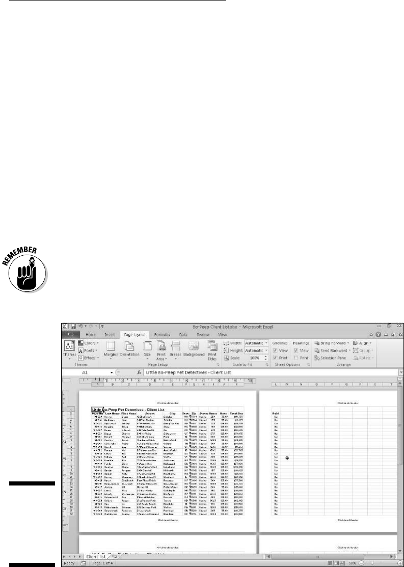
185
Chapter 5: Printing the Masterpiece
Because many worksheets are far wider than they are tall (such as budgets
or sales tables that track expenditures over 12 months), you may find that
wider worksheets page better if you switch the orientation from Portrait
mode (which accommodates fewer columns on a page because the printing
runs parallel to the short edge of the page) to Landscape mode.
In Figure 5-6, you can see the Print Preview window with the first page of a
report in Landscape mode in the Page Layout View. For this report, Excel can
fit three more columns of information on this page in Landscape mode than it
can in Portrait mode. However, because this page orientation accommodates
fewer rows, the total page count for this report increases from two pages in
Portrait mode to four pages in Landscape mode.
Putting out the print titles
Excel’s Print Titles feature enables you to print particular row and column
headings on each page of the report. Print titles are important in multipage
reports where the columns and rows of related data spill over to other pages
that no longer show the row and column headings on the first page.
Don’t confuse print titles with the header of a report (see “From Header to
Footer” later in this chapter). Even though both are printed on each page,
header information prints in the top margin of the report; print titles always
appear in the body of the report — at the top, in the case of rows used as print
titles, and on the left, in the case of columns.
Figure 5-6:
A Landscape
mode report
in Page
Layout
View.
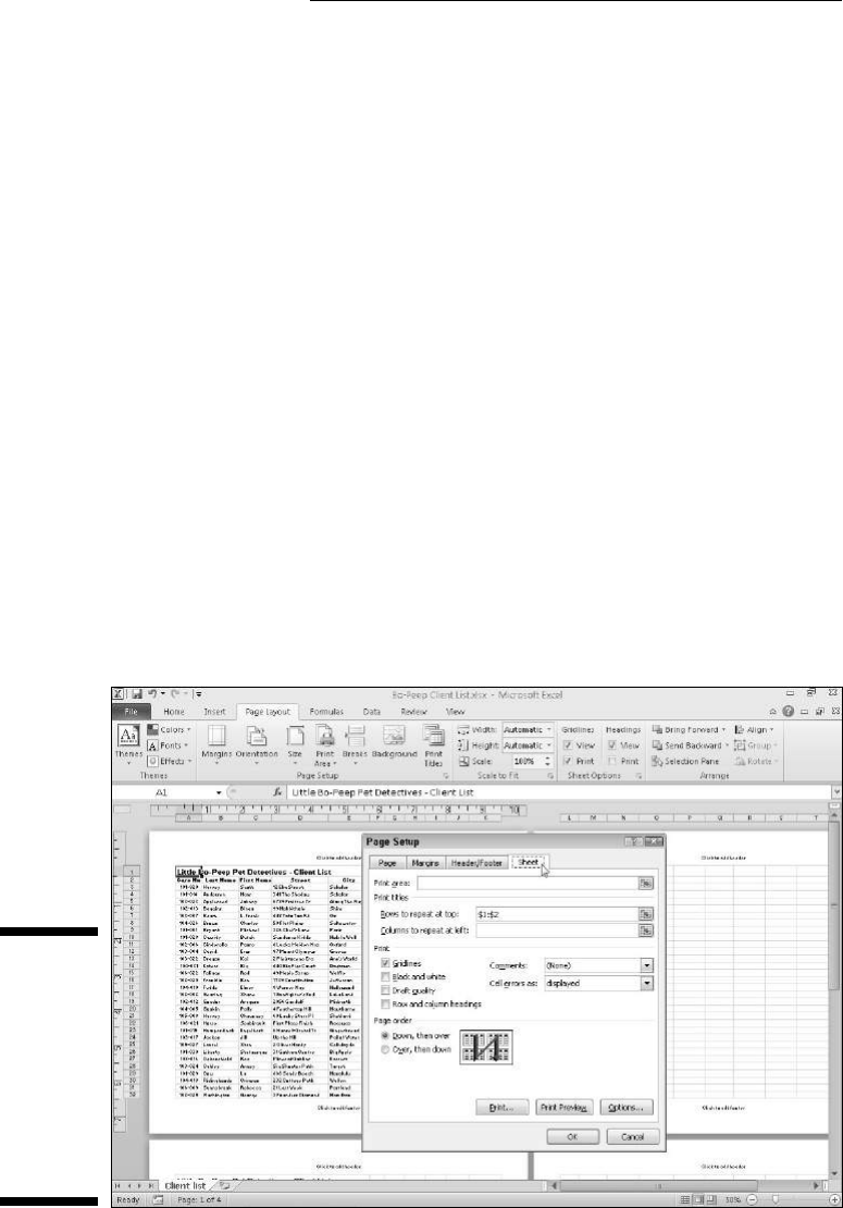
186
Part II: Editing without Tears
To designate rows and/or columns as the print titles for a report, follow
these steps:
1. Click the Print Titles button on the Page Layout tab on the Ribbon or
press Alt+PI.
The Page Setup dialog box appears with Sheet tab selected (refer to
Figure 5-7).
To designate worksheet rows as print titles, go to Step 2a. To designate
worksheet columns as print titles, go to Step 2b.
2a. Select the Rows to Repeat at Top text box and then drag through the
rows with information you want to appear at the top of each page in
the worksheet below. If necessary, reduce the Page Setup dialog box
to just the Rows to Repeat at Top text box by clicking the text box’s
Collapse/Expand button.
For the example shown in Figure 5-7, I clicked the Collapse/Expand
button associated with the Rows to Repeat at Top text box and then
dragged through rows 1 and 2 in column A of the Little Bo Peep Pet
Detectives – Client List worksheet. Excel entered the row range $1:$2 in
the Rows to Repeat at Top text box.
Excel indicates the print-title rows in the worksheet by placing a dotted
line (that moves like a marquee) on the border between the titles and
the information in the body of the report.
Figure 5-7:
Specify the
rows and
columns to
use as print
titles on the
Sheet tab
of the Page
Setup dialog
box.

* * * Free Preview End * * *
Purchase Required To Gain Total Access
Visit www.landlordleaseforms.com To Purchase Landlord Lease Forms Package